The 1: 100 000 Scale Topographic Mapping Program - Assisted by Technology

by Rod Menzies and Paul Wise, originally presented at the 2011 Conferenece, 100 Years of National Topographic Mapping, re-edited for the web 2022

Introduction

In 1960, the Commonwealth government’s Division of National Mapping and Royal Australian Survey Corps (RA Survey) were several years from completing Australia’s first topographic map coverage, the 1: 250 000 scale R502 series (77% of which were un-contoured). Nevertheless, based on experience and a vision to the future, these organisations proposed an improved map series that would have contours. It was expected that such a program would take 18 years to complete (Lines 1992). In 1965, after broad consultations on requirements and resourcing, the Commonwealth government decided that the program of topographic mapping should be accelerated with the object of completing mapping coverage of Australia at 1: 100 000 scale with contours at a 20 metre vertical interval, by the end of 1975 (Commonwealth Co-ordinating Group on Mapping Charting and Surveying 1983). The work on this National Topographic Map Series (NTMS) was to be undertaken by National Mapping and RA Survey, assisted by the States.

Each 1: 100 000 scale NTMS map was bounded by 30 minutes of latitude and 30 minutes of longitude (nominally 60km x 60km) where 1cm on the map represented 1km on the ground. The map projection was the Transverse Mercator using the spheroid and grid zones of the Australian Map Grid (AMG). Horizontal and vertical accuracy had to meet National Mapping Council standards.

From the outset, resources allocated to the NTMS program were never at the level required for the envisaged map publication schedule to be met. Thus the program faltered from inception and a more limited program of map publication at 1: 100 000 scale was adopted. Under this revised program, all map sheets would be compiled at 1: 100 000 scale but in the sparsely settled inland areas publication would be at 1: 250 000 scale. Elsewhere publication scale remained at 1: 100 000 scale. Notwithstanding the less than initially anticipated resource allocation, the NTMS program was hardly an inexpensive undertaking. The overall cost of the 1: 100 000 scale and 1: 250 000 scale maps produced under the program has been stated as $600 million (O’Donnell 2006).

Figure 1 shows the areas of responsibility for survey, compilation and map production as agreed in 1974. It further indicates that only 1: 250 000 scale publication would occur inside the thick line on the diagram. As this diagram with its thick red line of demarcation was printed in red, it became known as the Red Line diagram.

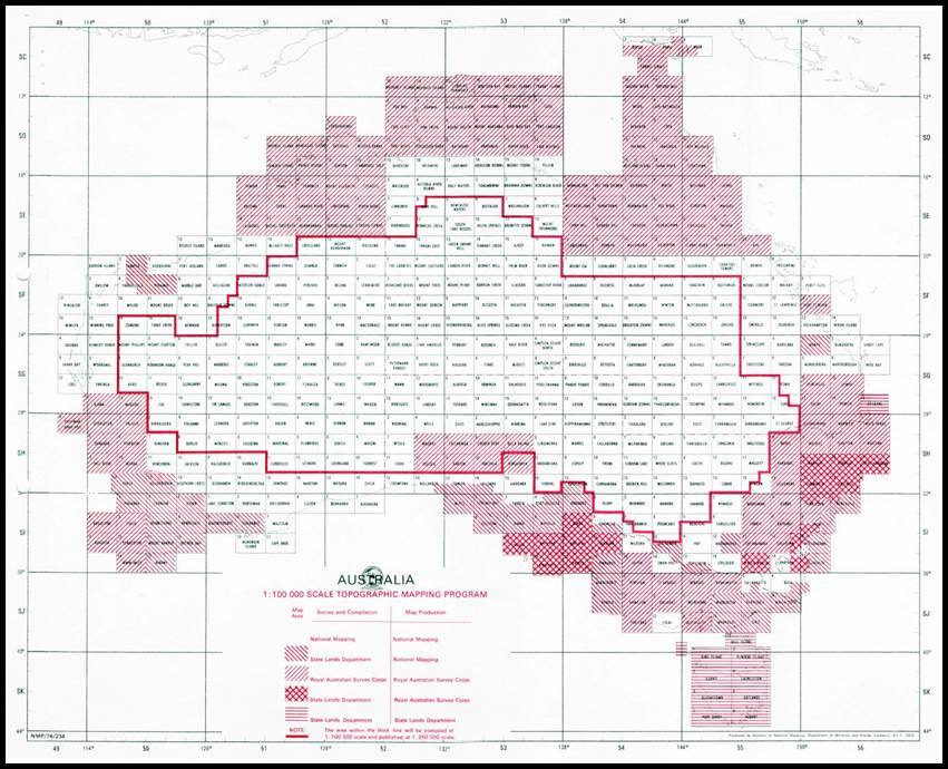
Figure 1 - 1: 100 000 Scale Topographic Mapping Program - the ‘Red Line’ diagram (Division of National Mapping 1974).

The National Topographic Map Series (NTMS) at 1: 100 000 scale comprised some 3 062 map sheets which were completed around 1988. Some 1 460 map sheets covering the more remote inland of Australia were only produced to the compilation stage (O’Donnell 2006). All 1: 100 000 scale compilations were used to derive new 1: 250 000 scale maps, gradually replacing the earlier R502 map series of the same scale. The 1: 250 000 scale NTMS program of 544 map sheets was completed in 1991.

To achieve this new program of mapping work and meet the standard of accuracy required, both National Mapping and RA Survey drew on the experience gained from completing the earlier R502 series 1: 250 000 scale mapping program. Both these organisations realised that data acquisition, processing and extraction had to be achieved as rapidly as possible; and the selected mapping component methodology had to be consistent such that expertise was developed and mistakes, if not eliminated, were minimised. New technologies in the form of aircraft fitted with data acquisition equipment could cover large areas and the emerging bureau services enabled access to computational speed and power for complex numerically based projects. Improvements in engineering, electronics and optics, allowed for new or enhanced capability. This paper reviews the major technologies applied to the aerial photography, horizontal and vertical control intensification, orthophotomapping and digital mapping components of the 1: 100 000 scale NTMS program and shows that role of these technologies in assisting the successful completion of the NTMS program.

Aerial photography

Australia’s first topographic map coverage, the 1: 250 000 scale R502 series, was largely based on 1: 50 000 scale aerial photography. This photography was captured by aerial cameras with wide angle (152mm) lenses. In the late 1950s, Wild Switzerland introduced the RC9 aerial camera with a superwide angle (88mm) lens and 230mm film format. A Wild RC9 aerial camera with its superwide angle lens is shown at Figure 2.

When flown at 25 000 feet above sea level (ASL), the RC9 camera produced photographs with a nominal scale of 1: 80 000. The number of 1: 80 000 scale photogrammetric models covering a 1: 250 000 scale map area was approximately 70% less than the number of 1: 50 000 scale models. (A photogrammetric or stereoscopic model generally consists of two aerial photographs that overlap by 60 per cent.) The reduced number of photogrammetric models to be controlled and used to plot the topography yielded flow-on economies for other components of the NTMS program (Division of National Mapping 1980). Thus the estimated overall cost-effectiveness of 1: 80 000 scale photography was greater than that indicated by the reduction in the number of stereoscopic models alone (Lines 1992). Given the magnitude of the NTMS program, it was necessary to capture such savings.

There was some concern that the RC9 camera (with its superwide angle lens) might miss imaging terrain on steep slopes receding from the camera towards the edge of the photo frame. Fortunately, there was little such steep slope terrain in Australia. Where steep slopes were present, appropriate planning of the photography flight lines allowed all terrain to be imaged. The superwide angle RC9 camera was introduced into the Federal mapping program in 1960. Its introduction commenced the systematic acquisition of aerial photography at 1: 80 000 scale with 25% side-lap and 80% longitudinal overlap (Lambert 1971). Introduction of 1: 80 000 scale photography did however cause some initial operational problems. The 230mm RC9 camera format meant that a photograph captured an area of about 19km x19km. Over such distances, earth curvature becomes significant and its effect had to be removed either by the mechanics of the stereoscopic plotter or in the production of the photographic media used in the stereoscopic plotter (the diapositive or transparent positive).

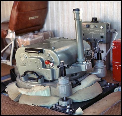
Figure 2 – Wild RC9 aerial camera with its superwide angle lens.

National Mapping was the provider of aerial photography for Commonwealth mapping purposes. In this capacity it made superwide angle Wild RC9 cameras available to commercial contractors. Between 1960 and 1975, private sector contractors flew systematic 1: 80 000 scale aerial photography over practically all of Australia. The exceptions were areas in Western Australia logistically difficult to reach (Manning 1988). Refer Figure 3. To standardise the provision of contract aerial photography, the National Mapping Council revised its Standard Specifications for Vertical Aerial Photography.

In 1976, in the light of successful United States’ experience with high altitude jet aircraft, National Mapping chartered a Gates Learjet 25C modified with a doorway camera pod. The Learjet was fitted with a then state‑of‑the‑art positioning system, the GNS 500A Omega VLF Global Navigation System (GNS). This system enabled the accurate transit of the photographic flight lines. For operations, National Mapping installed its own Wild RC10 aerial camera with an accompanying NF2K navigation sight. The RC10 was capable of using either a wide angle (152mm) or superwide angle (88mm) lens cone. The camera was fully accessible to the operator in flight, acquiring the photographs through the special optical glass ‘flat’ of the aircraft’s door pod and the navigation sight could back up the GNS position with visual sightings.

In 1976, North-South flight lines were adopted for RC10 superwide angle photography that had photo frames centred over map sheets and acquired at 45 000 feet above sea level; this configuration yielded photography at a scale of 1: 154 000. The 1976 capture program completed the outstanding desert areas of Western Australia. The photography was planned to enable an orthophotomap covering an entire 1: 50 000 scale map sheet to be produced from a single photo frame. However, problems were encountered with the final product. In particular, resolution was poor and the photographs had excessive tips and tilts that resulted from the roll and pitch of the aircraft (the short wing Learjet was slow to react to autopilot corrections in the thin atmosphere at 45 000 feet ASL).

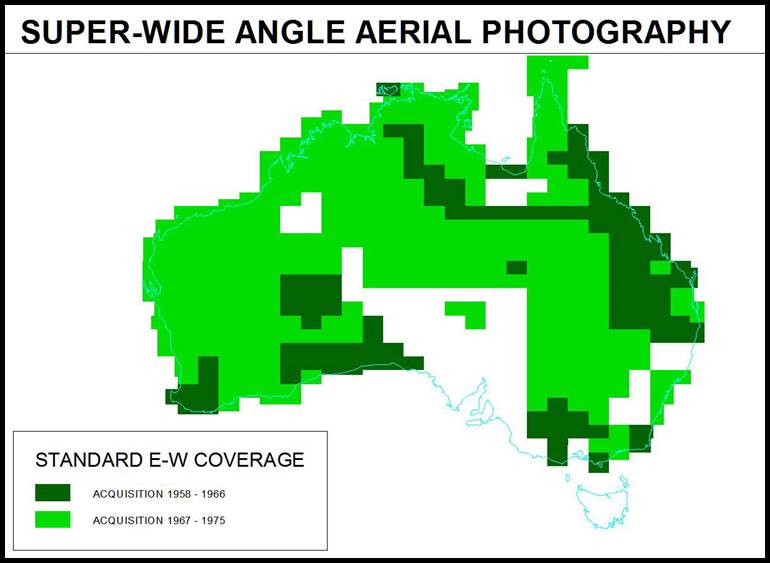
Figure 3 – Wild RC9 superwide angle aerial photography, 1958 – 1975.

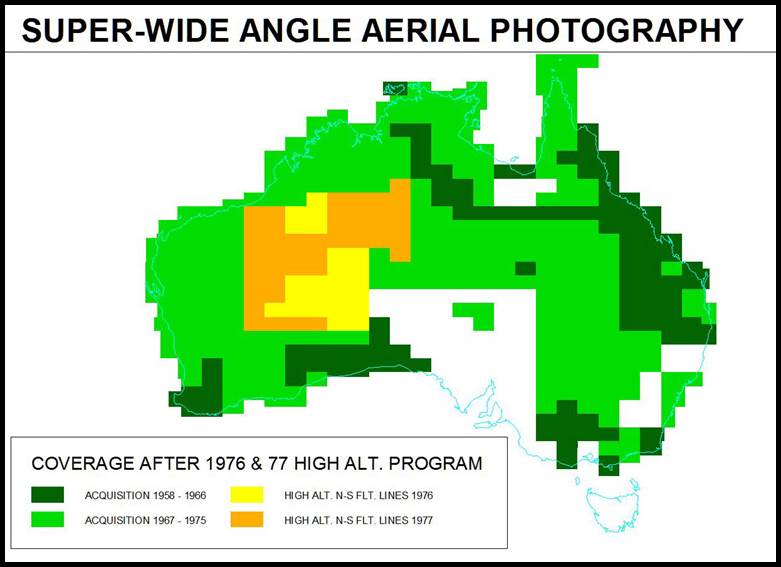
Figure 4 – Wild RC9 superwide angle aerial photography, 1958 – 1977.

High altitude photography was flown again in 1977. That year the Learjet was flown at 40 000 feet ASL; resulting in 1: 138 500 scale imagery. While the lower flight level improved the Learjet’s stability, single photo coverage of a whole 1: 50 000 map sheet was not obtained. Again problems similar to those in 1976 were seen in the final product but the coverage of Australia was completed. Refer Figure 4. The Learjet was chartered for the next 3 years and flown along the traditional East-West flight lines at 25 000 feet ASL. This obtained 1: 80 000 scale photography for the topographic mapping program. The speed and range of the Learjet enabled flying operations during optimum photographic conditions over extensive regions of Australia and thus maximised the area of successful photographic coverage per flying hour. RA Survey also experimented with acquiring and using high altitude photography for its future programs.

In 1982, National Mapping obtained its own aerial survey aircraft, a Cessna C421. This aircraft was capable of continuing 1: 80 000 scale superwide angle aerial photography acquisition for use in the remaining 1: 100 000 NTMS program.  The 1960 decision to adopt aerial photography acquired at 1: 80 000 scale by aerial cameras with superwide angle lenses to provide the topographic base for the national mapping program proved to be sound. Despite attempts in 1976 and 1977 to use smaller scale aerial imagery, the 1960 decision resulted in 1: 80 000 scale photography being acquired for a further 30 years and used for the majority of the NTMS program.

Horizontal and vertical control intensification

Until the 1960s, primary geodetic survey networks supplemented by identified survey marks that were positioned by astronomical observations provided the horizontal control for mapping. However, for the NTMS program each 1: 80 000 scale stereoscopic model of superwide angle photography had to be related to the ground and to each other to allow extraction of the required topographic detail at 1: 100 000 scale. Accordingly, the existing sparse horizontal control would have to be intensified; mainly through the use new airborne technologies.

Positional control for the 1: 80 000 scale photogrammetric models was achieved in a two stage process. Slotted template assemblies had already been used with great success to generate stereoscopic model control for the R502 series mapping program (Hocking 1987) so the required expertise and facilities already existed. The large loops of the geodetic survey, however, did not provide in themselves, sufficient control points to fix a template assembly to the horizontal positional accuracy for 1: 100 000 scale mapping.  Thus, a control network within each geodetic loop was required. The flatness of much of the Australian terrain made line of sight control intensification methods cumbersome so airborne solutions were sought.

In 1952, the then National Mapping Office with the then Bureau of Mineral Resources had undertaken a 1 mile to 1 inch mapping project in the Northern Territory using an airborne distance measuring system known as SHORAN; an acronym for SHOrt RAnge Navigation (Rabchevsky 1984). Appendix A contains a copy of a paper describing this project. SHORAN was an airborne system measuring to ground based equipment. The SHORAN ground equipment was bulky and housed in a van so any ground sites had to be accessible to those vehicles (in the days before four wheel drive vehicles were widely used). The wavelength used by the equipment for measuring also restricted operations to line of sight. The project’s success was marginal (Rimington et al 1954). For the NTMS horizontal control intensification program SHORAN did not provide a suitable option.

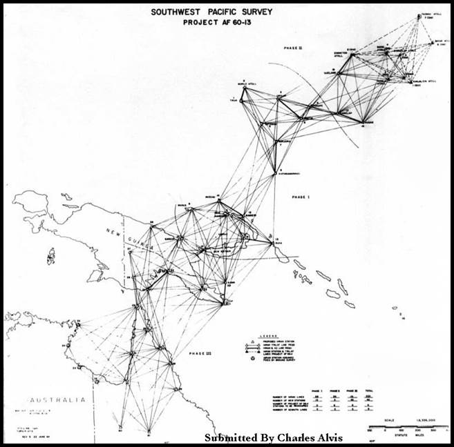
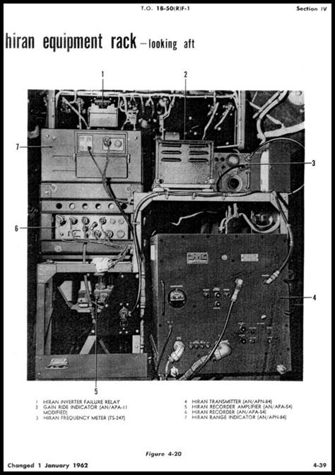
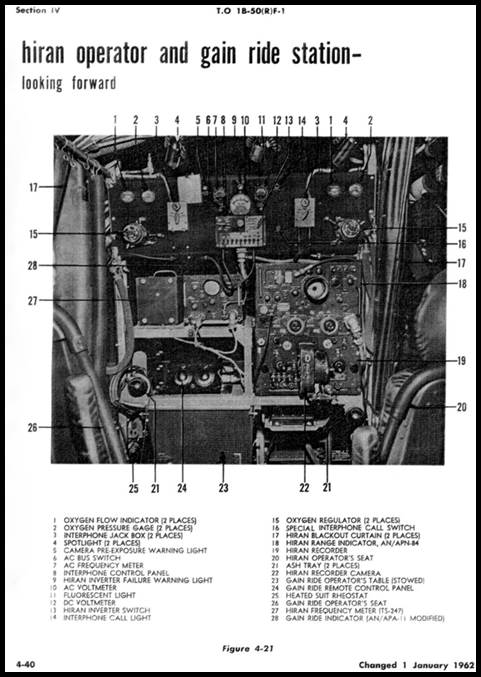
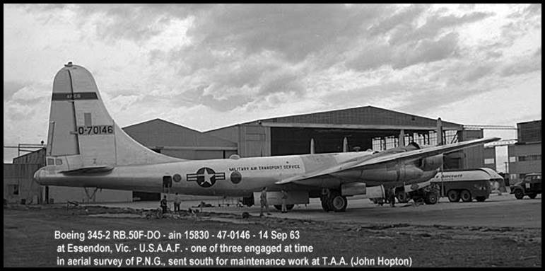
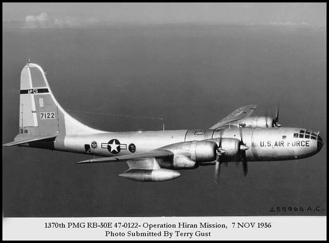
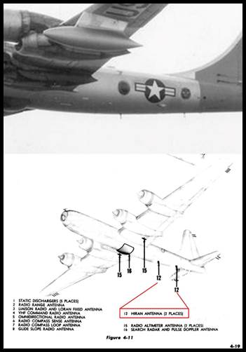
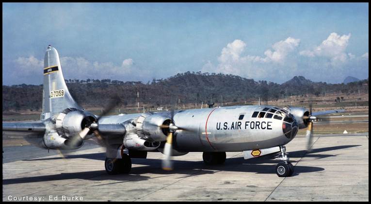
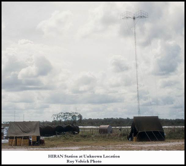
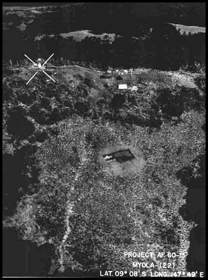
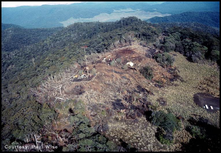
During 1962-1964, National Mapping field parties in Papua New Guinea (PNG) undertook (in co-operation with RA Survey amongst others) the geodetic survey of that territory. During that time a more expansive, survey operation was underway, namely the Southwest Pacific Survey. Appendix B contains further information on that operation. The Southwest Pacific project was accomplished by aerial electronic surveys that measured distances from an airborne station to each of two ground stations. The equipment used was called HIRAN. The name was a contraction of HIgh-precision shoRAN (Rabchevsky 1984), but also unofficially from HIgh frequency RAnging and Navigation. The US Air Photographic and Charting Service had developed HIRAN. Its improved accuracy over SHORAN was comparable with first-order ground triangulation over very long distances. However, the equipment was still bulky. Although line of sight was unnecessary HIRAN did not provide National Mapping with a suitable solution for intensifying horizontal ground control.

From 1957, the geodetic survey of Australia was rapidly extended with the Tellurometer electromagnetic distance measuring equipment (Ford 1979). Under a contract awarded by the United States Army Engineers Research and Development Laboratories in 1958, the South African firm of Tellurometer Pty Ltd developed an airborne system called Aerodist (McMaster 1980). The equipment offered the rapid and accurate long range extension of horizontal control either by:

· the line-crossing technique of distance measurement between two ground stations whereby the aircraft as an intermediate(albeit master) station was flown between the two (remote) ground stations several times,

· fixing an uncoordinated ground station from two coordinated ground stations using an aircraft and continuous trilateration,

· fixing two uncoordinated ground stations from two coordinated ground stations using an aircraft and continuous trilateration (Lines 1966).

The Aerodist ‘master’ units were fitted into the cabin of the aircraft. Each ‘master’ unit had its own unique frequency indicated by a colour code red, white or blue. This setup allowed simultaneous distance measurement on discrete frequencies. The ground units (called ‘remotes’) were similar to standard Tellurometers in that they were highly portable (Tellurometer Undated). Each ‘remote’ unit was also frequency colour coded, red white or blue. A ‘red master’ could only measure to a ‘red remote’ unit and so with white and blue. The minimum system of two master units (say red and white frequencies) could measure the distance simultaneously to two separate ground remote units, specifically to a ‘red remote’ and to a ‘white remote’. Refer Figure 5.

To permit greater operational flexibility, some ‘remote’ units were later modified as double back units that could be switched between two frequencies. For example, a red/white ‘remote’ unit could use the red frequency for the measurement of one line and then be switched to the white frequency for measurement of another line. The later use of three airborne master units allowed the distances to three separate ground remote units (using red, white and blue frequencies) to be measured simultaneously.

Figure 5 – Aerodist Master configuration and a Remote unit.

Based on its experience with the Tellurometer, National Mapping saw Aerodist as the solution to intensifying the horizontal ground control for the NTMS program. National Mapping’s initial Aerodist configuration comprised two master and four remote units. It was delivered and accepted in 1963. RA Survey had significant experience with the Tellurometer and also selected Aerodist for horizontal control intensification mainly in PNG. RA Survey received its set of Aerodist in 1964 (Coulthard-Clark 2000). RA Survey generally operated its system in a contract aircraft to fix an unknown point from two known points with the Aerodist remote on the unknown pointed vertically to establish height. National Mapping undertook some trilateration, fixing an unknown point from three known points, but the majority of new ground control for the NTMS was established by the line-crossing technique.

For the 1963 and 1964 field seasons National Mapping installed its Aerodist master units in a helicopter. For operational reasons, in 1965 this was changed to a chartered Rockwell Aero Commander 680E high wing aircraft.  However, the small cabin on this aircraft made it a tight fit for the equipment and operators. In 1966, a larger Rockwell Aero Commander 680FL (Grand Commander) was chartered and became the operational platform until the Aerodist measuring program was completed in 1974. By 1967, National Mapping’s Aerodist system had been expanded to three airborne master units with 6 remote units, 3 of which had been modified to switch to a second frequency. This configuration enabled almost daily measuring operations as ground based parties with the ‘remote’ units were often moved by helicopter to predetermined ground locations.  

The Aerodist master units in the aircraft were flown across the line between remote units at the ground stations (line-crossing technique) - see Figure 6a. The changing distances between the master and remote units were recorded on a chart recorder in the aircraft. For each line- crossing, aircraft and ground meteorological data were recorded for use in the final line-length reductions. Generally, National Mapping used the Aerodist system to measure distances between non-intervisible ground survey stations, building up a regular trilateration pattern of 1º (but sometimes 30') quads. The Aerodist survey configuration was basically a series of braced quadrilaterals of measured lines, linked to and contained within the existing geodetic network that formed discrete blocks of trilateration ‑ see Figure 6b.

Figures 6a and 6b – Diagrammatic view of the line-crossing technique and a typical Aerodist block adjustment.

Once all lines in the block were computed the block was adjusted by method of least squares to the surrounding geodetic control to obtain coordinates on the Australian Geodetic Datum for that network. The array of complex Aerodist computations could not have been achieved as quickly as it was without access to a computer service bureau. Data was punched onto cards and batch jobs were run through the CSIRO computing network; initially on a Control Data Corporation (CDC) 3200 computer but later on CDC3600 and 7600 computers.

Despite access to computing resources all initial strip chart reductions were done manually and entered onto proforma from which the punch cards were generated. In addition, instrument stand point and meteorological information from the associated ground stations had to be extracted from the applicable field books and incorporated. It was a very demanding, tedious and time consuming task and not without error. In an endeavour to automate data extraction and reduction from the strip charts recorded in the aircraft, the CSIRO Division of Land Research and Regional Survey developed a chart ‘reader’.

Purchased in 1966, the ‘reader’ converted the chart trace to a digital record on punched paper tape that allowed direct input to the computer. Ancillary data was punched onto cards and software was written for the complete reduction from the breakout of the line crossing chart through to the final spheroidal distance for a measured line. The system was run with moderate success in parallel with the manual reduction process for several years but because of increased mechanical and electronic problems with the reader it was eventually discarded in favour of manual reduction only.

As can be seen from the diagram of Aerodist block adjustments in Figure 7, Aerodist, in just over 10 years, supplied the majority of second order control required for the NTMS program. The real success of Aerodist only emerged in later years when a range of independent measurements revealed that Aerodist coordinates were accurate to better than 5 metres. The Division of National Mapping’s Technical Report 27 (McMaster 1980) provides details of the Division’s Aerodist program.

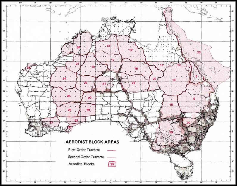
Figure 7 – Aerodist block adjustment areas.

Slotted Template Assembly

Combined Aerodist and geodetic networks provided sufficient horizontal control for a number of adjacent 1: 250 000 scale map areas to be selected as a ‘photogrammetric block’. An assembly of slotted templates was then used to graphically determine the positions of the horizontal control at the stereoscopic model level for that block (Lambert 1976). Refer Figure 8. As the slotted template technique is well documented elsewhere further discussion here is unwarranted.

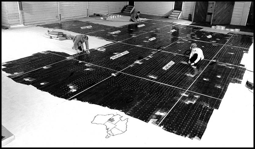
Figure 8 – Slotted Template Assembly (one of the largest produced by National Mapping).

As a result of work on the R502 mapping program, National Mapping had available a large number of staff with significant expertise in slotted template assemblies (Hocking 1967). For this reason, National Mapping used the slotted template technique for much of its NTMS program. Only later, when software, equipment and expertise became available, did National Mapping move to the analytical technique of numerical block adjustment which it ran in parallel with template work. In contrast, RA Survey chose to use the analytical technique from the outset.

Analytical technique of numerical Block Adjustment

As the computational speed and power of computers grew, analytical techniques evolved for calculating the horizontal position and the elevation of photo-control points. These photo-control points would allow each stereoscopic model to be oriented correctly relative to the ground and adjacent models. Unlike the slotted template technique which only intensified the horizontal control (leaving the vertical control to be determined separately), the analytical technique was able to manipulate both position and height within the same process. The areas of adjustment for horizontal control intensification by National Mapping are shown at Figure 9.

In principle, the numerical adjustment of a photogrammetric block entailed reading the spatial coordinates in a machine system of points common to adjacent stereoscopic models and the spatial coordinates of a selected number of ground control points. The machine system coordinates were related to the known ground system coordinates at the ground control points. The stereoscopic models were joined mathematically by adjusting their orientation and scale and then their co-ordinates transformed into the ground system using the observed ground control points. Subsequently, systematic, three dimensional, ground based coordinates were produced for all photo-control points in the block. The advantages of the numerical/analytical method were seen to be:

Greatly reduced requirements for vertical control, thus reduced both field work and compilation

Three dimensional coordinates were produced for each model join points and so avoided the need to identify or transfer separate horizontal and vertical model control points as with the slotted template method.

Greater accuracy due to lack of mechanical failings of graphical systems

Output was in the form of magnetic tape or punch cards suitable for automatic plotting of map base sheets. This was able to be readily integrated with adjacent blocks; either extended or amended and was suitable for further intensification of control for larger scale or special purpose mapping.

The tedious aspects of graphical methods were avoided.

Template marking, cutting and laying were replaced by machine observations and mathematical manipulations.

Lambert (1971) recorded that for an analytical block adjustment, RA Survey established control at the corners and mid top and bottom of unit photographic areas. These areas usually comprised blocks of 200 models and provided an additional checkpoint in the centre of the block. This gave a grid spacing of 75 km east/west and 50 km north/south. Vertical control was provided at the extremities and centres of each flight strip with additional control along the northern and southern edges of the blocks.

Figure 9 – Block Adjustments for 1: 100 000 scale mapping by National Mapping.

National Mapping’s approach was to establish horizontal and vertical control at the corners of units of about 120 models which usually constituted areas about 100 km² and numbers of these units were enclosed within the perimeter control for the block. The perimeter control for a block was usually the existing network of stations at either 1° or 30¢ spacing, with vertical control provided at a spacing of 4-6 models (60km) along all flight strips.

The difference in approach was largely dictated by the different block adjustment programs used by the two agencies and the requirements to meet the NTMS accuracy standard. While the majority of horizontal control intensification for the NTMS program was provided by slotted template assemblies, by the end of the NTMS program analytical methods had been adopted by National Mapping as the methodology for the future.

Adjustment programs

As mentioned above, National Mapping’s access to computing power was provided by service bureaus. However, from the 1960s the actual computer programs that harnessed this power were developed or modified to suit the organisation’s requirements by National Mapping’s own staff. The three most notable programs used were:

VARYCORD

First used in the geodetic adjustment of Australia in 1966 this program ran on a Control Data Corporation (CDC) 3600 computer (Lambert 1969). VARYCORD was replaced in 1972 by VARUDEL which ran on a later CDC6600 computer and produced the results in half the time (Bomford 1973). A version of VARYCORD was also used for adjusting Aerodist blocks where the distances and azimuths were weighted inversely to the length of the lines (McMaster 1980).

LEVELONE and LEVEL 2

These two programs were used in the national levelling adjustment. Originally written for a Control Data Corporation 3600 computer they were also converted for a CDC6600 (Roelse 1975). LEVELONE computed a least squares adjustment by observation equations of height differences in a network with one fixed origin. LEVEL 2 computed a least squares adjustment by condition equations. This later program combined five LEVELONE regional adjustments into one homogeneous net that was based on a single datum.

MODBLOCK

National Mapping’s numerical photogrammetric block adjustment program MODBLOCK along with FORMIT and MODSTRIP were written around 1972 and in later years ran on CSIRO's Cyber-76 computer. Model joins within each strip were tested by the strip formation program FORMIT. Joins of strips to ground control, where applicable, were tested by the strip adjustment program MODSTRIP. The final join of strips to each other and to ground control was performed by the block adjustment program MODBLOCK.

It is noted that for its numerical photogrammetric block adjustments, RA Survey undertook considerable work so that Schut’s polynomial and bundle adjustments would run successfully on their smaller, in-house Digital Equipment Corporation (DEC) PDP11/70 mini-computer .

Vertical control intensification

Irrespective of which method of horizontal control intensification was used, vertical control was also needed. To provide height information for each 1: 80 000 scale stereoscopic model it would be necessary to intensify the vertical control provided by 3rd order levelling loops. Attempts at vertical control information capture were made using barometric methods (ground and airborne) with some success but it was new, more accurate airborne technology that again proved to be the most cost-effective. However, a unique, semi-automated, ground based approach did impress the heads of both National Mapping and RA Survey when seen in 1963 in the United States.

Johnson Ground Elevation Meter

The Johnson Ground Elevation Meter was demonstrated to National Mapping and RA Survey in 1963. Refer Figure 10. Such were its capabilities that both organisations purchased one each. Both arrived in Australia in 1964. This machine was a modified General Motors Corporation (GMC), four-wheel drive van. It had automatic tyre pressure monitoring, four wheel steering and air conditioning (for the on-board electronic equipment rather than the crew). Its central feature was a special, smaller ‘fifth’ road wheel. A ‘bar’ ran between the front and rear axles with an electronic pendulum attached. The ‘fifth’ wheel accurately measured the distance travelled during operations by generating signals at a frequency proportional to the vehicle’s speed. Simultaneously, the longitudinal angle of the vehicle was continuously measured by the pendulum that generated a current proportional to the sine of the angle of tilt.  The on-board computer combined the two measurements and provided a paper print out of the height variation at any point along the vehicles traverse run.

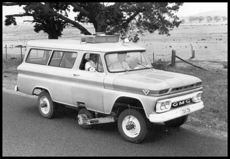
Figure 10 – National Mapping’s Johnson Ground Elevation Meter.

During a traverse operation, the height difference between a bench mark and the ‘fifth’ wheel was taken with a spirit level and staff. The vehicle was carefully driven to the next point where the height difference from the computer was noted. Then the level and staff were again used to measure the height difference between the ‘fifth’ wheel and the bench mark. Mathematical application of these three height differences provided the height of the second bench mark or a check on the original levelling. In practice, National Mapping found it best to start from an existing bench mark and drive to the next existing bench mark establishing as many new points as required as the traverse proceeded. The process was independently repeated on the return journey. After proportioning any misclose from the two ‘runs’, the average of the two independent heights for each point was then adopted.

Sperry-Sun Rand system manufacturers, claimed fourth-order levelling standard, 24 hours a day, seven days a week in all weather. However, these claims could not be met under Australian conditions largely due to the then quality of sealed road surfaces; the ‘fifth’ wheel required a relatively smooth surface to maintain accuracy. Nevertheless, National Mapping obtained results with an error of less than 3m in 80km travelling at 25kph when on reasonably good road surfaces.  Ground Elevation Meter traverses averaged 160km per day (Department of National Development 1965). Overall, between 1964 and 1974 around 5% of all National Mapping vertical control was obtained using the Johnson Ground Elevation Meter (Lines 1992). In flat country, where the sealed road system was reasonably extensive, the Elevation Meter demonstrated that a network of heights could be obtained which allowed contouring for 1: 100 000 scale mapping (Lines 1967). Nevertheless, airborne terrain profiling was to become the long term technology that supplied National Mapping’s vertical control at the stereoscopic model level.

Airborne Profiler Recorder (APR)

The Airborne Profile Recorder was developed in Canada in the late 1960s. APR, in the form of the Canadian Applied Research Ltd (CARL) Mark V, was bought to Australia by private enterprise and was first operated under contract to National Mapping in 1962 (Lines 1992). Also in 1962, RA Survey obtained its own system which was used by a contractor to fly profiles in PNG in 1963 (Coulthard-Clarke 2000).

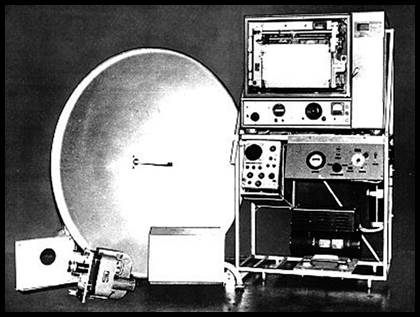
Figure 11 – CARL Mark V Airborne Profile Recorder equipment showing radar reflector left with 35mm camera in foreground and chart recorder top right.

Simplistically, the APR system was based on radar continuously measuring the aircraft-ground distance. This measurement was displayed as a pen trace on a continuous paper chart. This trace showed the terrain profile. Actual ground position of the profile was recorded by a vertically-mounted 35mm camera that exposed sequential, overlapping frames. The exposure of each frame caused a separate event mark to be recorded on the paper chart and thus related the ground location to the paper chart profile position. APR generally acquired terrain profiles in the common side-lap of the 1: 80 000 scale aerial photography with the 35mm frames used to transfer the required position of the chart height to the stereoscopic model.

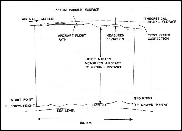
Figure 12 – Terrain profiling for vertical control.

Without knowing the height of the aircraft above some datum (Australian Height Datum), the profile heights were only relative. However, the accuracy of aircraft altimeters (and even later autopilots) did not allow the aircraft to maintain a sufficiently accurate set altitude along the profile. Therefore, a refinement was added; the hypsometer (later statoscope) or very sensitive altimeter. At profiling altitude, the hypsometer was ‘locked’ to that atmospheric pressure and along the profile measured any deviation from that initial reference pressure. These deviations were displayed by another pen trace on the chart and used to correct the final heights.

Unfortunately, the use of a pressure surface between datum checks added a computational overhead to the extraction of height values from the profiles. The initial reference (‘locked’) pressure can be considered to form a surface of constant pressure or isobaric surface. Such an isobaric surface is curved and while a small section can be considered as a plane, it is never horizontal. In 1947, Mr T.J.G. Henry of the Meteorological Division, Department of Transport of Canada, determined that the slope of the isobaric surface was directly related to the drift of the aircraft and could be calculated by the subsequently named ‘Henry correction’. The amount of Henry correction at each height point could be calculated as a proportion of distance travelled during the profiling flight. Refer Figure 12.

Operationally, to set up the hypsometer datum and calculate the Henry correction, the following procedure was adopted by the contractor. After take-off the aircraft would climb to an operating altitude of around 10 000 feet. Flying over the airstrip the aircraft had just left, the hypsometer would be ‘locked’ at that pressure altitude and then the aircraft would set off to fly the profiles. After each profiling flight the aircraft would return and re-fly the airstrip before landing. (Airstrips were almost always used as datum points as their open and relatively flat surfaces made good radar targets and were connected to the AHD network). All the way through the flight, drift would be measured to allow the necessary inputs to the Henry correction. The before and after flight over the airstrip allowing any misclose of the Henry correction to be proportioned. The airstrip’s AHD height would allow all profile heights to be related to AHD. Lines (1967) recorded that individual APR heights were not in error by more than 25ft but when used as model control these errors ‘averaged out’ and greater accuracy was achieved.

Final APR heights were derived from the mathematical sum of the terrain profile height modified by the hypsometer correction, Henry correction and misclose. All APR height computations were done manually. The complexity of the Henry correction along with the extraction of flight information and scaling of distance made the process lengthy, intricate and highly error prone. Gross checks at different stages were able to detect most erroneous calculations but from time-to-time a problem was only revealed when a photogrammetric model could not be oriented correctly in the stereoplotter. As production was halted until the problem was resolved APR height computation was a far from ideal process.

As experience grew with the use of APR heighting in the mapping process its limitations became more obvious. The radar system operated in the 3 cm band and required an antenna reflector, 1100mm in diameter. The physical size of the antenna and associated electronics required a large aircraft. (A Lockheed Hudson ex World War 2 bomber aircraft was used by the contractor. The antenna was housed in the old bomb bay section covered by a fibreglass screen so not to detract from the aircraft’s aerodynamics). In addition, at operating altitude, the radar illuminated an area of terrain about 50m in diameter. Where the relief changed height quickly, the radar produced an ‘averaging effect’ that reduced the accuracy of individual height points (Lines 1970).

The whole APR flight, from datum to profiling and back to datum had to be almost continuous to provide profiles of the required accuracy. Further, ideal flying conditions had to prevail and equipment failure had to be almost non-existent. However, over time, as the mechanics of the pens, chart recorder, frame camera and the early electronics became unreliable and productivity suffered accordingly. APR was last acquired for National Mapping in 1970 in central Western Australia.

WREMAPS I

As the problems and limitations of the APR system became more apparent, a replacement airborne technology was looked for and came in the form of a purpose built laser based system (Penny 1970). This system was built by the then Weapons Research Establishment (WRE), Department of Supply in South Australia. Its official name was WREMAPS 1 but it was generally known in National Mapping as the Laser Terrain Profiler (LTP). Refer Figure 13. RA Survey took delivery of a later model, WREMAPS II in 1973. This later system had improvements in design and data capture that suited RA Survey’s operational requirements (Penny 1972).

Figure 13 – National Mapping’s Laser Terrain Profiling equipment.

A laser overcame the beam-divergence and accuracy problems of radar. The LTP used a continuous wave Argon Ion laser that operated at a wavelength of  0.5mm. LTP distance measurements taken at 50/sec were accurate to better than 3cm and its narrow beam only illuminated an area of terrain less than half a metre in diameter. Furthermore, the system was able to be installed in a smaller modern, fixed-wing aircraft.

The terrain profile from the LTP was output on an ultra-violet sensitive, 7 channel, continuous chart recorder and ground position was simultaneously recorded by a 70mm strip camera. The 70mm camera acquired a continuous record of the ground position of the profile. A timing code recorded on both the film and chart enabled a location on the 70mm film to be related to its position on the chart profile.

The 70mm strip camera imaged the terrain by means of a slit and incorporated automatic exposure control. A dichroic mirror reflected some of the light being imaged by the camera on to a screen visible to the operator. Across this screen appeared to move a series of equally spaced lines. These lines were generated by only being able to view part of a rotating disc engraved with a spiral. It was part of the operator’s role to keep these lines travelling across the screen at the same apparent speed as the terrain below and at the same time compensate for drift of the aircraft. As the disc was driven by the film transport motor, by adjusting its speed the operator synchronised the film speed with the aircraft’s ground speed and ensured equal longitudinal and transverse film scales.

Initially a statoscope, a refinement on the earlier hypsometer, was used to measure and output the deviations from the isobaric surface. Later, the statoscope was replaced by the Barometric Reference Unit (BRU) designed and built by WRE.

The LTP became operational in National Mapping in 1970 after being installed in a chartered Rockwell Aero Commander 680FL (Grand Commander). In 1977, it was moved into National Mapping’s own GAF Nomad 22B, where it operated until 1979. In 1980, due to RA Survey having problems with WREMAPS II, National Mapping acquired profiles for that organisation with its WREMAPS I. This was the last time WREMAPS I was used operationally.

The introduction of LTP enabled flying operations to be revised. The smaller ‘laser footprint’ meant that individual bench marks on the 3^rd order levelling loops could be used as datum rather than airstrips. The more numerous bench marks enabled more frequent datum checks and removed the need for the Henry correction and reduced the complexity of height computations. The error in any individual height obtained from LTP seldom exceeded ±2m (Wise 1979). Like APR before it, the LTP profiles were flown down the side-lap of the 1: 80 000 scale aerial photography and reduction of the required height points was undertaken manually. To help eliminate errors in the tedious reductions, each height was independently calculated twice. The Division of National Mapping’s Technical Report 26 (Wise 1979) provides details of the Division’s WREMAPS 1 profiling operations.

Figure 14 shows that LTP in about 10 years of operation along with APR in some 8 years of operation provided the majority of the vertical control for the NTMS program. However, with the emergence in the early 1980s of a possible requirement to meet 1: 50 000 scale map specifications with 10 metre contours, a more accurate profiling system was required. The new system needed to be smaller and lighter for installation into National Mapping’s Cessna 421C aircraft and had to incorporate digital data capture and processing.

Laser Airborne Profiling System (LAPS)

The Laser Airborne Profiling System (LAPS) was a refinement of the concept of the earlier WREMAPS profilers. LAPS used the 70mm strip camera and BRU from those systems. A pulsed laser capable of 1cm accuracy was the heart of the system and PC based data capture and verification plus digitally based office processing allowed for height computations to emerge more rapidly. Vertical control for the NTMS program had been completed by the time LAPS became operational but further details may be found in Manning and Menzies (1988) and Manning (1989).

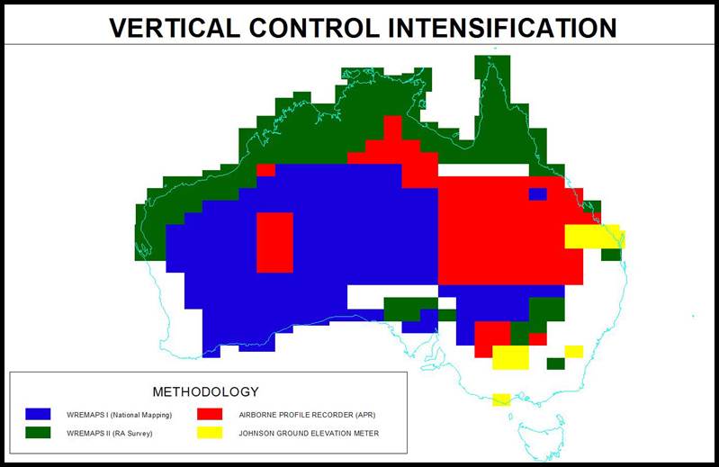
Figure 14 – Vertical control intensification for 1: 100 000 scale mapping.

Orthophotomapping

To extract the information necessary for a topographic map, a 1: 80 000 scale stereoscopic model was placed in a stereoplotter and the control previously discussed used to orient it horizontally and vertically. Thus the information subsequently extracted was located correctly and at the required map scale. The three-dimensional view provided to the operator of the plotter also allowed the terrain to be represented by tracing its contours at 20m intervals. Stereoplotting was a very time consuming task requiring great skill and visual acuity. While having some in-house capacity, National Mapping mainly used a panel of contractors to undertake this task.

As computer assisted technology advanced in the late 1960s it was foreseen that a ‘rapid mapping’ solution might lie in the form of ‘orthophotomaps’. Additionally the push for topographic information to support burgeoning minerals exploration and development required the detail of the aerial photograph. However, such detail needed to be in a format from which accurate coordinates could also be derived so that mining claims/mineral rights could be accurately referenced. The orthophotomap seemed to provide a solution for this pressing requirement.

An orthophotograph is an aerial photograph in which the terrain, earth and camera related distortions have been removed. Therefore features in the photograph are truly positioned and to scale. Put together as a mosaic, such corrected photographs formed a new map product - the orthophotomap. National Mapping generated orthophotomaps by two different processes depending on the relief of the terrain within the area that was being mapped.

Figure 15 – Wild B8 Stereomat, Zeiss Jena Topocarts and Zeiss Oberkochen SEG V rectifier.

In areas of low relief and plains country, where by this definition relief is not an issue, the earth and camera related distortions were removed using a process known as ‘single photo rectification’. A Zeiss Oberkochen SEG V rectifier was used for this purpose following its receipt in 1971. Refer Figure 15. A single photograph was projected by the SEG V onto its tilting table. The distance between the projector lens and the table was set to achieve the correct scale. Material, on which previously determined control points at the required scale had been plotted, was then placed on the table. The table was tilted such that the predetermined control points on the projected photograph and table were aligned; thereby correctly orienting and scaling the projected image. The control material was then removed and replaced by photographic paper onto which the projected image was captured. After this image was developed an orthophotograph emerged. By joining the requisite number of orthophotos together (mosaicing), also providing some enhancement of drainage and culture and adding a grid and surround the orthophotomap was produced. The process did not generate contours. National Mapping met demand for contour overlays for its orthophotomaps largely from contract stereoplotting sources.

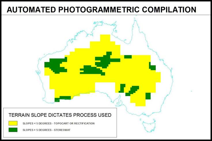
Figure 16 – Diagram indicating process used for orthophotomap production.

In more complex terrain, Wild B8 Stereomats (for country of high relief – refer Figure 16) and Zeiss Jena Topocarts (for country with medium relief) were used. Refer Figure 15. National Mapping, at full operation in the early 1970s, had two of each type of machine running around the clock seven days a week. National Mapping received its first Stereomat in January 1968 and a second machine followed in 1969. Its two Topocarts arrived in 1970. When National Mapping moved into digital mapping these four machines were the first to be incorporated into the computer network as their electronics generated the requisite digital co-ordinate outputs. By the mid‑1980s changed methodology was adopted and standard B8 and Kern PG2 stereoplotters were retro-fitted with superior encoders (an encoder converted plotter movement into electronic signals that formed digital co-ordinates). After these developments, the Stereomats and Topocarts were antiquated and were subsequently sold off.

The Wild B8 Stereomat emerged from the combined expertise of Wild Switzerland (optics) and Raytheon USA (electronics) and for the first time automated much of the old manual stereoplotting operations. After two film diapositives (that formed a stereoscopic model) were oriented in the Stereomat a small area was continuously auto-correlated as the machine scanned successive strips across the model. The auto-correlated areas (actually small orthophoto segments) were imaged onto photographic film and contours at a predetermined interval could be added or recorded as separate digital data. In theory at least, once scanning commenced the operator was superfluous. However, such situation only lasted until, for whatever reason, auto-correlation was lost and the operator was required to establish it again for the machine! In practice, these machines were operated manually with an operator constantly monitoring the machine’s operation to reduce the instances of loss of auto-correlation. Height data was continuously collected as the photogrammetric model was scanned and this data was recorded on magnetic tape. These data tapes were later computer processed to generate contours which were downloaded on an automatic data plotting table.

The Topocart was more like the traditional stereoplotter in that an operator was required to retain correlation but imaged the orthophoto segments to film like the Stereomat. However, the Topocart had the versatility of variable scan widths which reduced production time in areas of intermittent relief. In the type of terrain where this equipment was used, there were normally not a great number of contours. Thus it was not such a tedious task to fully contour each photogrammetric model manually after scanning. As the contour was traced by the operator the line emerged from a plotter on a side table.

By the late 1970s the requirement for orthophotomaps had declined and traditional line map users preferred the line map to the orthophotomap. While there had been some experimentation with combined line and orthophotomap, the majority of civilian map users preferred the traditional product. All othophotomaps were eventually converted to line maps; the last being completed in 1988.

Digital Mapping

As computers and their peripherals evolved through the 1960s and into the 1970s their use for mapping was being developed. Digital mapping technology provided the capacity to produce maps at any scale on any projection quickly. This capacity included the production of special maps with superfluous detail filtered out. In addition, a further advantage of digital mapping was seen in its capacity to provide information to users in a digital form that could be combined by computer with other user information for planning studies and various other potential applications.

In the early 1970s, RA Survey decided to move into the digital era and by 1976 accepted its AUTOMAP I system that was supplied by SYSTEMHOUSE (Canada) (Royal Australian Survey Corps 1978). RA Survey’s AUTOMAP II followed in 1984 (Coulthard-Clark 2000).

While aware of the advantages of ‘going digital’, National Mapping’s path was, however, handicapped by the ongoing resource constraints and the risk averse bureaucratic practices of the time. Nevertheless, in 1977 the Commonwealth Public Service Board supported a proposal to gradually introduce computer assisted topographic mapping techniques to replace the conventional methods. Over the next few years, the necessary equipment and expertise was accumulated and importantly included software based on RA Survey’s AUTOMAP system and also supplied by SYSTEMHOUSE. By both agencies having AUTOMAP software, future digital data exchanges were greatly facilitated.   

Digital compilation in National Mapping’s Dandenong Office got underway around 1982. Also in 1982, after National Mapping’s Canberra office received and accepted a computerised, precision, flatbed Kongsberg plotter. This plotter allowed digitally derived reproduction material (a prelude to the printing process) and small scale mapping products to be generated in the Canberra office. Figure 17 refers.

Figure 17 – Digital capture system (left) and precision data plotter (right).

The topographic map compilation process required the acquisition of digital data from aerial photographs mounted in stereoplotting instruments fitted with encoders. However, if compilation material already existed it was digitised (either in-house or by contract). The data was then edited, verified and assembled into 1: 100 000 areas and additionally generalised to 1: 250 000 scale specifications for publication. All data was then written to magnetic tape for further processing in National Mapping’s Canberra office. Map production in Canberra involved using the compilation data from the magnetic tape to plot the final reproduction overlays of map sheets on the precision plotter. Repromat at 1: 250 000 scale (and 1: 100 000 scale where required) was produced as well as any editing, generalisation, verification and plotting of the digital data for mapping at smaller scales.

The naming of features on a map was a very important aspect of the mapping process (Kennard et al 1977). Selecting the features to be named along with ensuring their correct spelling and attributes (type font, point size and case) was a very time consuming and error prone process. As computer assisted cartography evolved at National Mapping, a system to automate the extraction and typesetting of feature names for mapping purposes was developed.

A gazetteer of Australian map feature names was originally compiled from the 1: 250 000 scale R502 map series. It was later updated, expanded and sorted into alphabetical order within 1: 100 000 map sheet areas. To enable automatic feature selection based on order of importance to be made, a hierarchical system was established for groups of features, such as populated places, drainage networks, relief features etc. By setting up rules as to what hierarchical levels were required for a particular scale of map only the feature names applicable would be selected. For a small scale map, for example, only the highest (i.e. most important) hierarchical levels of city, river etc names would be selected by the software. The file of selected feature names and attributes could be further processed by an automatic type setting machine. Such a machine read the file and generated the feature names in the associated type font, point size and case on negative film. This film was then contact printed to positive, reverse reading, stripping film. As required, the feature names could be extracted from the stripping film and stuck down on a clear plastic overlay in relative proximity to their associated feature with the knowledge that spelling and attributes were correct.

Digital Mapping and completion of the NTMS Program

The Hermannsburg (5450) 1: 100 000 scale map sheet was the first sheet to be fully compiled by stereoplotting and table digitising by National Mapping. Significantly, it was the last map required to complete its NTMS program. These important aspects of the Hermannsburg sheet saw it being endorsed by the Federal Minister for Administrative Services, the Hon. Stewart West MP in October 1987 (Moody 2010).

While digital mapping did not greatly impact the NTMS program, this technology and the NTMS program itself became the ‘springboard’ for the next generation of mapping (O’Donnell 2006).

Concluding remarks

For much of the last half of the 20th Century, Australian mapping agencies (Federal and State) struggled to record our country in three dimensions. Such a mapping record was well understood as being necessary for the effective planning, development, management and defence of our nation. The history of this endeavour shows that achieving this three dimensional topographic record was too often hampered by competing public priorities and attendant resourcing constraints. Nevertheless, it is likely that in coming generations, history might acknowledge that it was the initiative, skill, perseverance and co-operation of those same agencies which successfully introduced, adapted and utilised a range of new technologies to complete each agency’s part of this record. Today, this achievement is evidenced by the three-dimensional record contained in the maps of the NTMS program. The maps and data products produced from this program provide the cornerstone of a comprehensive national data infrastructure (O’Donnell 2006).

Acknowledgements

The authors acknowledge the many former Natmap and other agency people for contributions to this paper and in particular:

Mr Laurie McLean for his critical review of the paper,

Messrs Kevin Moody and John Allen for their recollections and advice,

Mr Milton Biddle for information on the Johnson Ground Elevation Meter, and

the late Bob Goldsworthy whose writings and photographs were a valuable resource and whose contribution to Natmap was exceptional.

References

Bomford A.G. (1973) Geodetic Models of Australia, Department of Minerals and Energy, Division of National Mapping, Technical Report 17, ISBN 064 2943753.

Commonwealth Co-ordinating Group on Mapping Charting and Surveying. (1983) Initial Report of CCGMCS, 1982, NM 83/153.

Coulthard-Clark, C. D. (2000) Australia’s Military Map-Makers: The Royal Australian Survey Corps 1915-96, Oxford University Press, 2000, ISBN 0 19 551343 6.

Department of National Development. (1965) Summary of Activities 1963-65, Department of National Development.

Division of National Mapping. (1974) 1:100,000 Scale Topographic Mapping Program, NMP/74/234, 1974.

Division of National Mapping. (1980) Development of Aerial Photography in Australia, Cartographic Instructions, Section 1, Instruction 2 : Issued 1980.

Ford, R. A. (1979) The Division of National Mapping’s part in the Geodetic Survey of Australia, The Australian Surveyor, vol. 29, no. 6, pp. 375-427; vol. 29, no. 7, pp. 465-536; vol. 29, no. 8, pp. 581-638.

Hocking, D.R. (1967) Photogrammetric Planimetric Adjustment, Colloquium on Control for Mapping, University of New South Wales 22-24 May, 1967.

Hocking, D.R. (1987) Mapping Data and the National Mapping Programme, The Globe, no. 28, pp. 31-37.

Kennard, R.W. and Stott, R.J. (1977) An Automatic Name Selection and Typesetting System, Division of National Mapping, Technical Report 22.

Lambert, B.P. (1969) Geodetic Survey and Topographic Mapping in Australia, The Australian Surveyor, vol. 22, no. 7, pp. 515-528.

Lambert B.P. (1971) Super-wide Angle Photography and Orthophotomapping in the Australian Federal Mapping Programmes,  50 Years Wild Heerbrugg 1921-1971, pp. 68-72.

Lambert, B. P. (1976) Topographic Mapping in Australia: Development 1945-1975, Australian Cartographic Conference (Adelaide), Section 13, pp. 1-14.

Lines, J.D. (1966) Aerodist in Australia, 1963-64, The Australian Surveyor, June 1966, pp.733-751

Lines J.D. (1967) Control Surveys for 1:100,000 Mapping, 5th United Nations Regional Cartographic Conference for Asia and the Far East, Canberra, March 1967.

Lines, J.D. (1970) Developments in Airborne Profiling :  Laser Terrain Profiling Equipment, 6th United Nations Regional Cartographic Conference for Asia and the Far East, Iran, 1970.

Lines J. D. (1992) Australia on Paper – The Story of Australian Mapping, Fortune Publications, Box Hill.

Manning, J. (1988) From Aerial Photography to Remote Sensing – a History of Aerial Photography and Space Imagery Acquisition in Australia, Technical Papers Australian Cartographic Conference (7th : Sydney), pp. 300-318.

Manning, J. (1989) The AUSLIG Laser Airborne Profiling System, Australian Survey Congress, Hobart, pp. 1-9.

Manning, J. and Menzies, R. W. (1988) Vertical Control for Australian Topographic Mapping, Australian Survey Congress, Sydney, pp. 117-137.

McMaster C. G. (1980) Division of National Mapping Aerodist Program, Technical Report 27.

Moody, K. (2010) Personal correspondence.

O’Donnell, I. (2006) The State of National Mapping 400 Years On, 400 Years of Mapping Australia, 2006, Darwin, CD-ROM.

Penny, M. F. (1970) An Airborne Laser Terrain Profiler, Department of Supply, Australian Defence Scientific Service, Weapons Research Establishment, Salisbury, South Australia, Technical Note OSD 116.

Penny, M. F. (1972) WREMAPS II : System Evaluation, Department of Supply, Australian Defence Scientific Service, Weapons Research Establishment, Salisbury, South Australia, WRE-Technical Note-811 (AP).

Rimington, G. R. L., McCarthy, F. E. and Robinson, R. A. (1954) Application of Shoran to Australian Mapping, Cartography, December 1954, vol. 1, pp. 7-20.

Rabchevsky, G.A.(Ed.). (1984) Multilingual Dictionary of Remote Sensing and Photogrammetry, American Society of Photogrammetry, Falls Church: Virginia, USA.

Roelse, A., Granger, H. W. and Graham, J. R. (1975) The Adjustment of the Australian Levelling Survey 1970-71, Department of National Development, Division of National Mapping, Technical report 12. – 2nd edn.

Royal Australian Survey Corps. (1978) Position Paper : AUTOMAP - March 1978, National Mapping Council, 29th Technical Sub-committee Meeting, Bendigo,1978, Item 5.3.12.

Wise P. J. (1979) Laser Terrain Profiling, Division of National Mapping Technical Report 26.

Tellurometer. (Undated) AERODIST : An Airborne Tellurometer System, Tellurometer Pty Ltd Brochure.

Appendix A

Application of Shoran to Australian Mapping

Approval for reproduction by the

Surveying & Spatial Sciences Institute (SSSI)

is greatly appreciated

Application of Shoran to Australian Mapping

by G. R. L. Rimington, F. E. McCarthy and R. A. Robinson

Abstract

Shoran used to fix position of scintillometer flights, and control for planimetric maps, in uraniferous areas in the Northern Territory. Overseas use. Australian experiments. Reasons for using Shoran. Description of Shoran equipment. Method of fixing geographical positions of Shoran beacons and mapping control points. Selection of control points. Plotting of scintillometer results. Analysis of results. Lecture given 29 July 1954, by G. R. L. Rimington, Chief Topographic Surveyor, National Mapping Office; F. E. McCarthy, Supervising Geophysicist, Bureau of Mineral Resources; and R. A. Robinson, National Mapping Office.

Introduction

The first Australian application of Shoran to control mapping was in the project at present nearing completion in the Rum Jungle area; of the Northern Territory. Accurate planimetric maps were required to serve as a base for prospectors' charts, at one mile to an inch, showing radioactive anomalies obtained from airborne scintillometer surveys conducted by the Bureau of Mineral Resources.

Overseas use

Shoran along with other forms of radar has been used overseas to some extent in connection with triangulation and mapping. However, reports on the routine use of radar for mapping in other countries are very few, although extensive experimental work has been reported from England. In general, there are three instances where radar has been used in a routine mapping project overseas and in order of importance they are :

1. Establishment of a network of geodetic survey in Canada using Shoran.

2. Overwater triangulation by the United States using Shoran.

3. Extensive mapping at medium scales in Africa by means of Gee H. (British type of radar).

The Canadian network is very extensive and when completed, it is hoped this year, will give control points extending over most of Canada from latitude 50° N. to latitude 66° N. and from longitude 120° W. to longitude 70° W. The axial length of the chain of triangles will be 5,500 miles and will form a huge arc having considerable connections to five geodetic bases.

The overwater triangulation - or as it is often called, Trilateration - has been used in the United States to connect islands to the main geodetic chain. Generally, Shoran operations in the United States have been, as in Canada, confined to the establishment of basic control.

In Africa, British organizations have carried out a good deal of work establishing minor control for mapping operations at medium scale, but no comprehensive reports are available on the results obtained.

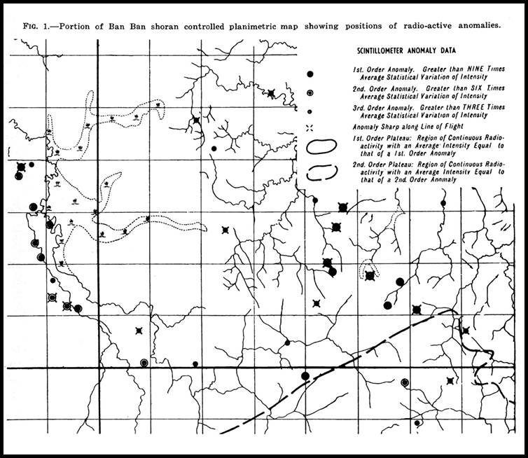
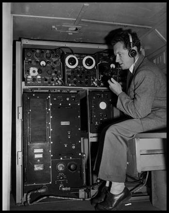
Figure 2 – Shoran receiver                                                     Figure 3 – Beacon equipment

Australian Experiments

The first experiments in the application of Shoran to mapping in Australia, arose from the formation of a Subcommittee of the National Mapping Council, whose task was to report on the possibility of using this means of accelerating the mapping programme.

This committee arranged with the Commonwealth Scientific and Industrial Research Organization, which was in possession of a number of units of equipment, to carry out tests.

In line with most other countries, the tests were devoted to the establishment of basic control. An ideal test area existed in N.S.W. where it was possible to measure all six lines of a quadrilateral, the position and lengths of which were fixed by existing triangulation, This quadrilateral was located with points at Condobolin, Tamworth, Sydney and Canberra, the lines varying in length from 158 to 311 miles.

Mr. J. Warner of the C.S.I.R.O. carried out the tests and reported them in the Australian Journal of Applied Science, Vol. I, No. 2, 1950. His conclusions are interesting and are quoted :

"This method of distance measurement using the line-crossing technique gave an average accuracy of roughly one part in 15,000 when measuring lines of 160 to 310 miles in length. The greatest source of error is the radar equipment that was used and is associated with signal strength. It is considered that by suitable modification to the equipment, in particular to the receivers, this signal intensity error could be reduced to within 10 feet. If this were done, it is likely that the overall accuracy of the technique would improve to about 1 part in 50,000.

"An improvement on this latter figure would be impossible without extensive improvements to the radar equipment. In addition, a thorough investigation of the problems of atmospheric refraction would be necessary."

Figure 4. KEY DIAGRAM. 1. Shoran controlled parallel flight lines. 2. No. 1 Shoran beacon. 3. No. 2 Shoran beacon. 4. Shoran pulses. 5. Radio-active deposit. 6. Area covered by scintillometer. 7. Radiations. 8. Scintillometer instrument panel. 9. Instrument recorder. 10. Instrument panel. 11. Shoran transmitter. 12. Sharon receiver. 13. Instrument recorder. 14. Instrument camera. 15. Instrument panel. 16. Shoran distance indicators. 17. Shoran transmitter. 18. Communications equipment. 19. Beacon transmitter. 20. Beacon receiver monitor. 21. Handwheels. 22. Repeater motor dials. 23. Cathode-ray oscillograph. 24. Distance indicating dials. 25. Shoran receiver.

Whilst these tests were being carried out, a representative of the National Mapping Office acted as an observer, to try and gather some idea of the economics of the whole problem. The facts that he gathered in regard to the operation of the equipment were such that the Subcommittee on Radar could not recommend the method as an economic proposition.

It was felt by the Subcommittee that the demands on money and manpower required to use Shoran for mapping purposes would be beyond the very tiny resources of the existing National Mapping Office. Regretfully, the "seven league boots" of Shoran were placed in cold storage, and the classic methods of mapping control were continued.

This "cold storage" did not last very long (two years), as the discovery of uranium in Australia altered the economic aspects. It was not so much the discovery of uranium that so largely altered the position, but rather the development of the airborne scintillometer. This instrument revolutionized the search for uranium, and also brought with it extensive demands for accurate mapping and its associated control.

Use of Shoran Equipment

Search for Uranium

One of the functions of the Bureau of Mineral Resources is to conduct airborne surveys in the search for uraniferous deposits. These surveys are carried out using a D.C.3 type aircraft in which the detecting equipment is housed along with navigation and auxiliary equipment.

The navigation aids include a set of Shoran equipment and a radio altimeter along with the standard navigation instruments such as compasses, radio compass, barometric altimeter, etc.

The equipment used to detect radioactivity from the ground flown over is the scintillometer. This is a recent development and is much more sensitive than any arrangement of Geiger-tubes which may be used. Nevertheless, the scintillometer has limitations when used in an aircraft. The most serious of these is the inability to detect gamma radiations from a "point" source deposit of radioactive ore when the distance, in air, between the scintillometer and the source is more than 800 feet. Because of this limitation the aircraft carrying the scintillometer is flown at height no greater than 500 feet above the ground; and to obtain adequate coverage of an area suspected of containing radioactive minerals, the aircraft is flown along parallel flight lines one-fifth of a mile apart. (Figure 4.)

Navigation

It is not possible to navigate an aircraft flying 500 feet over wooded country along parallel flight lines of such close spacing by normal means of navigation. Consequently, some radio or radar means of navigation is required. The various types of radio navigation aids were investigated, and it was decided to use Shoran. The reasons for this choice were:

(i) that the Shoran equipment was readily available on loan from C.S.I.R.O.;

(ii) that the ground beacon units were more portable and required less power than beacon for any other system;

(iii) that the system would give the desired degree of accuracy for positioning of the aircraft.

It was realized that the Shoran equipment operated on wavelengths which would restrict the range of the system to line of sight operations, but the advantage of using Shoran outweighed those of any of the long wave length systems such as Raydist and Decca.

Shoran Mapping Control

The purpose of using the Shoran equipment on these surveys is twofold. Firstly, to enable the pilot to fly the aircraft accurately along pre-selected flight lines, and secondly that the aircraft position must be known at all times so that any areas showing abnormal radioactivity could be plotted on a map to enable follow-up ground parties to locate and investigate the areas. As there were virtually no accurate maps of the Northern Territory in which to plot these recorded anomalous areas, the National Mapping Office was approached to prepare maps.

This Office was willing to undertake map production provided that the Bureau of Mineral Resources supplied the control. The existing meagre control in the Northern Territory consisted of a single line of triangulation running approximately south from Darwin. This was insufficient to control maps over the areas to be flown by the aircraft, so the Bureau undertook to provide Shoran controlled aerial photographs for the purpose of laying down maps.

By basing the control runs on the same Shoran beacons as controlled the scintillometer runs, close relationship between the anomalies and the planimetric detail would be assured.

The area required was already covered by photography for mapping purposes, so it was not necessary to use the British system of fixing each exposure by radar. Instead, a Williamson F24 vertical camera was installed in the aircraft and control runs of overlapping F24 photos were flown. These runs were flown round the perimeter of each one mile area and north and south across the centre.

It was then a simple matter to transfer the principal points of these photos on to the plotting photographs to obtain control points.

When an area has been selected for airborne survey, a reconnaissance party is sent into the area to select accessible high points on which the Shoran ground beacons can be located. The mobile units carrying beacon equipment are moved on to the selected sites. Because of the limitation of line of sight operation of the Shoran equipment, the sites for the beacons are selected on the highest accessible points.

The bulk of the ground beacon equipment also limits the possibilities, as the sites must be accessible to the van carrying the equipment.

In this project, these two factors far outweighed other considerations. It was impossible to select the beacon sites so that good intersections could be obtained over the whole area.

Description of fixing the geographic positions of the beacons is given later.

After the positions of the beacons had been determined flight lines were laid down for the scintillometer survey and flight lines for the Shoran controlled aerial photographs for map control purposes were selected. It may be pointed out that in many cases the flight lines for map control were not always such as to give the best results, but the expediencies of the survey necessitated that the control flight lines were flown when possible and from existing beacon set-ups.

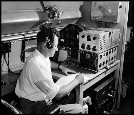
Figure 5 – Instrument panel

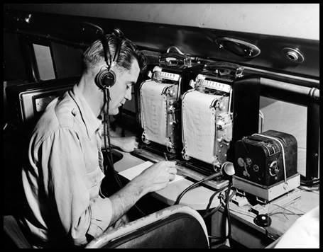
Figure 6 – Instrument camera

Usually about five control lines were flown over each one mile area, three in a north-south direction and two in an east-west direction. The control flights were undertaken from an altitude of 5,000 feet, and during these flights an F24 type aerial camera was triggered to take photographs at 10 second intervals. The instrument camera (14 on diagram) in the aircraft was triggered simultaneously with the F24 camera and it photographed a panel of instruments (15 on diagram) in the aircraft including the Shoran distance indicators (16 on diagram). By this means the distance of the principal point of each F24 photograph from each beacon was ascertained.

The Shoran distance indicators read directly in miles to the nearest one-hundredth of a mile. These indicators are operated by electric servo-mechanisms remote from the Shoran equipment.

The Shoran Equipment

Radar Responder System

The Shoran system is essentially a radar responder system. A transmitter (17 on diagram) carried in the aircraft transmits pulses of short duration. These pulses are received at the ground beacon, are amplified, delayed for a predetermined short time, and made to trigger the beacon transmitter (19 on diagram). These re-transmitted pulses are picked up on the Shoran receiver in the aircraft. The time taken for the round trip of these pulses travelling at the speed of light is a measure of the distance of the airborne unit from the beacon. The measured time is converted automatically into a distance in the airborne unit, and shows the distance of the aircraft from one beacon.

A single transmitter in the aircraft transmits pulses on two frequencies, namely, 230 and 250 mc/s. There is a switching mechanism in the airborne unit which switches the tuning on the transmitter so that it sends out a series of pulses on one of these frequencies for each alternate one-tenth of a second period, and then on the other frequency for the intervening periods of one-tenth of a second. The transmitter is pulsed at a repetition rate of 931 095 pulses per second (an important figure) and the duration of each pulse is 0 000002 seconds. That is, for alternate periods of one-tenth of a second, approximately 93 pulses are transmitted on a frequency of 230 mc/s and are picked up by the receiver at beacon No. 1 which is tuned to receive them. On the each intervening period of one-tenth of a second duration, approximately 93 pulses are transmitted on a frequency of 250 mc/s and are picked up by the receiver at beacon No. 2, which is tuned to frequency of 250 mc/s. Both beacons re-transmit the pulses on a frequency of 300 mc/s, to which frequency the receiver in the aircraft is tuned. The pulses received by the aircraft receiver are amplified and made to appear as deflections on a cathode-ray oscillograph (23 on diagram). This cathode-ray oscillograph has a circular time base which is triggered at the same rate as the transmitter. That is, during the interval between outgoing pulses from the transmitter, the luminescent spot on the face of the cathode-ray oscillograph traces out a complete circle of about two and one-half inches diameter. A reference pulse appears as a small outward deflection on the top centre (12 o'clock position) of the time base, and the pulses received from the beacons appear as deflections outward from the centre and inwards towards the centre of the circle. When the aircraft transmitter is transmitting on 230 mc/s the output of the receiver is switched, by the same switching mechanism as mentioned above, so that it is coupled to the cathode-ray oscillograph such that the output of the receiver will deflect the cathode beam away from the centre of the tube, consequently the responder pulses from the beacon No. 1 will appear as short duration "pips" on the outside of the circle. And in the same way, during the next succeeding one-tenth of a second period, the output of the receiver is switched so that the pulses coming from beacon No. 2 will appear as "pips" on the inside of the circular time base.

If the marker "pip" at the top of the circle appears at the same instant as the transmitter pulse is sent out, then a measure of the distance (or time) around the circle to the responder "pips" would be a measure of the distance of the aircraft from the beacons. As it is not possible to measure such distances accurately, much more elaborate arrangements for measuring these distances (or times) are incorporated in the equipment.

Quartz Crystal Oscillator

The accuracy of the Shoran equipment depends upon the ability of the system to measure small intervals of time very precisely. If the distance from the aircraft to the beacon increases by the smallest measurable distance, 0.01 miles, the travel path of the transmitter pulses increases by double this amount, 0.02 miles. The time taken for a radio wave travelling at a speed of 186,219 miles per second, to traverse 0.02 miles is 0.000,000,107 seconds, consequently the Shoran equipment must be capable of measuring time correct to this small interval.

The heart of the airborne measuring equipment is the time measuring device, or the quartz crystal oscillator. This operates on a frequency of 93,109.5 cycles per second, and generates a sinusoidal voltage. This alternating voltage is divided electronically in two stages to frequencies of 9,310.95 and 931.095 cycles per second respectively. After amplification, the sinusoidal voltage of the latter frequency is squared and made to produce one electrical pulse of two microseconds duration per cycle.

This pulse is fed on to the cathode-ray oscillograph and forms the marker or reference pulse.

Goniometer

A portion of the 931.095 c/s sine wave voltage is passed through the goniometer where the phase of the alternating voltage can be changed, continuously and accurately. This voltage is passed then on to a pulse forming network and a pulse is produced at exactly the same part of the cycle as the reference or marker pulse on the un-phased alternating voltage curve. This pulse is amplified and used to trigger the transmitter. By rotating the goniometers (changing the phase of the alternating voltage) the time separation between the transmitted pulse and the reference or marker pulse can be altered by very minute amounts. Sixteen revolutions of the goniometer shaft changes this interval by a time of 0 000,010,7 seconds, the time interval equivalent to a range of one mile.

The Shoran operator has a means of rotating the shaft of the goniometer and in doing so alters the interval of time between the transmitted and marker pulses so that this interval is exactly the same as the time required for the round trip of the transmitted pulse to the beacon, and back. If the transmitted pulse precedes the marker pulse, then the incoming signal or pulse will arrive at the same instant as the reference pulse is produced, and both pulses will appear on the same position on the cathode-ray oscillograph. The function of the Shoran operator is to turn the goniometer so as to keep the received pulses and the marker pulses aligned on the cathode-ray oscillograph. There are two goniometers in the unit, one for ranging to each beacon. The shafts of the goniometer are geared mechanically to the distance indicating dials (24 on diagram) which show the range of each beacon to the nearest 0.01 miles.

The frequency of the crystal oscillator, therefore, is controlled to within narrow limits.

It was stated above that the luminous spot on the cathode-ray oscillograph traced out a circle in the interval between transmitted pulses. This is true when the range switch is in the "100 mile" position, i.e. when the distance around the time base represents a distance of 100 miles. When the range switch is in the positions "10 mile" and "1 mile", the distances represented around the circle on the cathode-ray oscillograph are 10 miles and 1 mile respectively. The 100 mile and the 10 mile ranges are used only to enable the operator to align the pulses when first setting up. The procedure for the operator is to have the range switch initially in the 100 mile position and align the received pulses, then change to the more accurate 10 mile range and align the pulses again and finally to switch to the most accurate one mile range, and keep the pulses "tracking". The assumption is made that the distance of the aircraft from each beacon is known, from other sources, to the nearest 100 miles.

Aided Layer Equipment

It would be arduous work for the operator to turn the goniometers continuously to keep "tracking" the aircraft as the distances of the aircraft from the beacons are changing continuously. For example, for an aircraft travelling at a speed of 180 miles per hour directly away from a beacon, the range from the beacon is increasing at the rate of 3 miles per minute. The goniometer "tracking" this beacon would need to be rotated at a speed of 48 revolutions per minute. To lighten the work of the operator an "aided layer" unit has been added. There are two handwheels (21 on diagram) on the front of the aided layer which are coupled through a differential gear train by an electromechanical system to the shafts of the goniometers, and the operator can keep the pulses aligned on the cathode-ray oscillograph with only small movements of the handwheels.

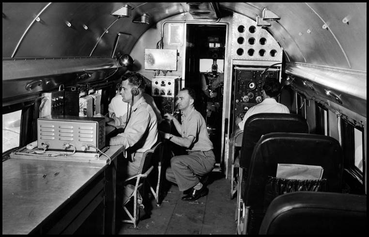
Figure 7 – Aircraft interior

Limitations and Source of Error

There are limitations to the accuracy of the Shoran, some of which may be solved in time. The more important of these are listed below:

(1) The use of the equipment is restricted to line of sight operations.

(2) The accuracy is dependent to some extent on the size of the received pulses at the beacon and aircraft receivers. It is not possible with the present equipment to incorporate automatic gain control in the receivers so that pulses out of the receivers are all of the same magnitude, irrespective of strength of the received signals. This comment applies particularly to the airborne receiver.

(3) The speed of transmission of radio waves has been taken as constant. It is known that this varies with atmospheric conditions. If the result achieved warranted it, a check could be made of the atmospheric conditions, and small corrections applied to the measured distances.

(4) Errors in measured distances can be caused by operator fatigue. Errors from these sources are thought to be small. Changing of operators at short regular intervals overcomes this to a great extent.

It is intended that the above will give the broad outline of the operation of the Shoran equipment. No attempt has been made to include small but important features or refinements incorporated in the equipment. For further details consult reference 1 at end of this article.

Mapping from Shoran Controlled Photographs

Beacon Site Fix

Each beacon site position was computed from a series of Shoran distances obtained from triangulation stations as illustrated in Figure 8. Ground survey parties from the National Mapping Office re-observed those parts of the old network which were required and established two further stations to fix these beacons sites' geographical positions.

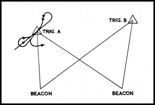
Figure 8 – Beacon fix

The aircraft flew a pattern over trig. A, taking vertical F24 photographs synchronized with the instrument panel camera. The distances to the principal point of each photograph were measured from both beacons. The triangulation stations were marked on the ground and could be identified on the photograph so that this Shoran distance could be adjusted for the distance from the triangulation point to the principal point of the photograph.

On each such flight, several (average four) triangulation points were covered from the same pair of beacons to provide a series of triangles with known sides and two positions known. From these the beacon positions could be computed. The flying pattern over each triangulation point was such that tilt and drift errors were minimized.

Office Computations

The information obtained from the B.M.R. field operations was collated and handed over to the N.M.O. for application. Briefly, this consisted of:

(1) The F24 photographs and their Shoran co-ordinates for obtaining the position of the beacon sites.

(2) The overlapping F24 photographs for each control run.

(3) The instrument camera films containing the data for each F24 photograph.

(4) A series of log sheets on which the instrument panel data had been tabulated and correlated to the F24 photographs.

The initial requirement was a set of co-ordinates for each beacon so that the control points based on them could be computed.

For each beacon there was a series of distances to various points, these points being the principal points of vertical photographs taken over triangulation stations of known position. Each Shoran distance was adjusted to allow for the distance from the principal point of the F24 photograph to the triangulation point. All references to Shoran distances apply to the figures obtained after the height and curvature correction has been applied.

To obtain approximate positions for the beacons and thus subsequently for each individual control point, an accurate one inch to a mile grid was constructed, and all triangulation points in the area were plotted. Trial co-ordinates for each Shoran beacon were then scaled from the intersection of the arcs of the known Shoran distances.

From these co-ordinates, bearings to each triangulation station were computed, thus providing a computed bearing and a Shoran distance from each triangulation station to the beacon position being computed. A series of positions were computed from these bearings and distances, the co-ordinates of the beacon being obtained graphically from position lines through these computed points. This position is a close approximation and further computing refinements could be used if necessary.

Examination of the results shows appreciable residual errors. Of all the eleven beacons fixed in this manner, the position line which was farthest from the final adopted value for that beacon was 85 yards away. There were two of more than 70 yards, one of 60, two of 50, and so on down the scale, the best of the worst rays being only nine yards from the adopted position. A mean of the residual errors in the rays to each beacon varied between a maximum of 51 yards and a minimum of six yards.

Errors of this magnitude for the control points for this type of mapping are tolerable, but for the beacon sites on which all the other controls are based, greater accuracy should be demanded.

Cross-over Checks

This term has been applied to the check made between the positions obtained from each run, where two or more control runs intersect. As no previous evidence was available as to the reliability of Shoran control applied in this manner, it was considered prudent to carry out these checks. The results proved them to be necessary.

Their main purpose was to check between the Shoran co-ordinates of intersecting runs, making a comparison between Shoran positions, and the ground positions respectively, of the principal points of several photographs from each run. Also, when the control runs were flown, some mechanical difficulties were encountered in the intervalometers of the F24 and instrument cameras. This meant that although the cameras were synchronized, occasional difficulty was experienced in equating these two on the instrument panel. This relationship or equivalence could be established from the cross-over checks.

Three F24 photographs were selected from each run at the intersection, and the principal points transferred on to the K17 plotting photographs. The relative ground positions of these principal points were then determined by a photoscale radial line plot.

The relative Shoran controlled positions of these same points were then determined from a graphical position line plot, using trial point co-ordinates scaled from the one inch to a mile grid mentioned above.

The Shoran positions (open circles in Figure 9) were plotted at a scale of 1:31,680; and the radial line plot (positions shown as filled in circles) was at a scale of approximately 1:30,300. These two plots were superimposed, the relative positions shown as in Figure 9. Any errors in equivalence were immediately apparent. In Figure 9 those numbers in brackets show the positions obtained from the log sheets. The equivalence was corrected and the true position plotted as shown. Closer comparison was then made to detect any small irregularities between the intersecting runs.

In every case there were small differences in both azimuth and position. These differences were meaned out and an arbitrary position was adopted for that photograph which was to be used as a control point. From the Shoran plot the small adjustments to be made to the bearing and distance from each beacon were then scaled off.

Two sets of rectangular co-ordinates for the control point could now be obtained from the bearing and distances from each beacon controlling it. These two positions were plotted on a grid (usually at a scale of one inch equals ten yards) and a graphical solution obtained from position line arcs through them. The intersection of the position lines was adopted, and the rectangular co-ordinates of the control points scaled directly from the grid.

Selection of Control Points

Immediately after receipt from the B.M.R., all the F24 photographs in the control runs were charted on to composite one mile to an inch mosaics of the area. These mosaics had previously been compiled from those K17 photographs which were being used in the snap compilation.

From these mosaics, a very clear appreciation of the position was possible. Owing to the priorities placed on specific maps in the project, it was necessary to complete the areas singly and in a specified sequence. Great care had to be taken, therefore, in the selection of control so that the detail would match along the edge of adjoining maps. Usually in projects of this nature, several areas are assembled at once, but the order of priorities precluded such a scheme in this instance. The only alternative, therefore, was a high density of control, selected so that cantilevering of the slotted template assembly beyond this control was kept to an absolute minimum.

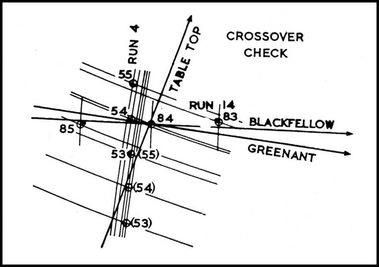
Figure 9 – Cross-over checks.

The first consideration, then, in selecting the individual F24 photographs to be used in control was that they should be outside the edge of the area being assembled. Where the control runs were not suitably situated to satisfy this condition, it was generally possible to control that edge by adopting a row of photo-points from a previous assembly. The next consideration was the condition of the template slots through the control. A well-conditioned six-ray intersection was to be aimed at in each case, and the F24 photograph most closely fulfilling this condition was adopted.

Initially, to provide a severe test on the accuracy of the control 20 points were used for each one mile area. These were evenly spaced around the perimeter control runs and along the centre key.

Those F24 photographs to be used for control could be selected directly from the composite mosaics, where all requirements could be considered.

No control point was computed until the equivalence for that section of the control run had been established by cross-over checks.

The computation for a control point is a simpler version of the cross-over check. In this case only the control photograph and the adjoining F24 photographs on either side are involved. The principal points of these three F24 photographs are transferred to the K17 photographs and radially plotted as before, at photo scale, to obtain the relative ground position. The relative Shoran positions are computed and plotted as before, using the Shoran co-ordinates of the control photograph to scale off a trial point. These Shoran positions were plotted at 1:31,680.

When the Shoran plots and the radial plots were compared, slight discrepancies were apparent each time. Arbitrary adjustments to the bearing and distances were made as in the cross-over check, and a graphical solution obtained.

Compilation of Maps

The control required for each map was completed in accordance with the priority order, each slotted template assembly being plotted as the control became available.

The maps were drawn from slotted template assemblies by the N.M.O. using the normal compilation procedure. Owing to the discrepancies between the template assembly and the computed positions of the control points, each area had to be considered individually, and those control points considered least likely to be correct were discarded.

The planimetric maps at one mile to an inch were drawn to standard military specifications, and astrafoil copies handed to the B.M.R. for the addition of their information.

Plotting of Scintillometer Results

Concurrently with the completion of the base maps by the N.M.O., the Bureau of Mineral Resources had been plotting the radioactive anomalies. To facilitate the plotting of this information, a series of Shoran lattices or grids was constructed.

A lattice was constructed for each one mile area, and for each pair of beacons controlling the airborne scintillometer survey of that area. Each lattice consisted of a network of concentric arcs centred on each beacon and spaced at intervals of one-fifth of a mile.

Each flight line on the scintillometer survey was plotted on the lattice directly from the corrected Shoran co-ordinates for each exposure of the instrument camera. Reference to the scintillometer graph then enabled the radioactive anomalies to be plotted along these flight lines.

The lattices were drawn at a scale of one mile to an inch, and the radioactive anomalies could be transferred directly to the base map with the correct relation to the planimetric detail retained.

Names of the features and marginal notes were then added, and the map prepared for publication in two colours. The topographic base was printed as a ghosted grey background, with the radioactive anomalies overprinted in black.

Analysis of Results

When the cross-over checks were plotted, varying differences between the Shoran coordinates of each run were revealed. The maximum difference in position between two intersecting runs was approximately 250 yards, and the greatest difference in azimuth over the sections plotted was about 6 degrees. However, these were exceptional cases, and the average difference was approximately 70 yards, and less than one degree in azimuth.

These discrepancies indicate that there are definite limitations to the use of Shoran in this manner, but with several refinements in procedure much better results can be expected.

A total of 142 control points was computed and tested by slotted template assemblies. In the early assemblies, where twenty points were used per one mile area, up to 50 per cent of the points had to be discarded. However, when the density of control was relaxed to 13 points per area, the percentage of discards was considerably reduced without any loss in the rigidity of the template assembly. In one assembly only one of the control points had to be discarded.

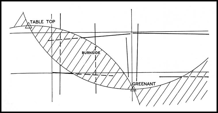
Figure 10 – Diagram showing “lens” of critical angle intersection.

The greatest factor limiting the accuracy of the control on this project was the siting of the beacon positions. The two main factors influencing their choice have already been mentioned, namely, line of sight scintillometer requirements and bulk of beacon equipment. A large percentage of the control runs were of doubtful value as the rays from the Shoran beacons controlling them cut at too small an angle to give an accurate intersection. For accurate results, the angle of intersection should be between 30 and 150 degrees. As can readily be seen from Figure 10, only those sections of the control runs inside the circles, but not within the "lens" between the circles, will satisfy this condition. In more accessible country the beacon sites could be selected to control the area being mapped, so as to satisfy the above condition with a consequent improvement in accuracy. If necessary, additional beacon sites could be used if those for the control s are not suitable for the scintillometer flights. The additional effort required would be more than offset by the improved accuracy.

The reliability of computing the position of the Shoran beacons from Shoran distances is also open to doubt. The results obtained showed appreciable residual errors in the rays from the triangulation stations fixing the beacons. Errors of 30 or 40 yards in the position of a control point can be tolerated in this type of country, but the beacon sites should be fixed much more accurately than this, as all other control points depend on these values. Until such time as the reliability of the method has been proved, and also to test the method, the beacon sites should be fixed by ground survey methods.

In common with all aerial photography, the effect of tilt was an important factor. At the flying height for the control runs, 5,000 feet, a tilt of three degrees displaces the principal point approximately 90 yards from the plumb point. An error of this magnitude is excessive, and can be eliminated only by perfect flying in ideal conditions. No obviously tilted photograph should be used as control.

A comparison between the overlaps of the F24 photographs and the Shoran intervals between successive exposures revealed small irregularities which materially affect the accuracy of control. These irregularities could be due to tilt or to the failure of the Shoran operator to keep the "pips" in coincidence. The task of the Shoran operator is far from easy, and even with frequent changes it becomes very fatiguing. A repeater Shoran tube on the instrument panel would provide a check on the operator, and any photographs where the "pips" were separated could be instantly discarded. However, several technical problems at present make this impracticable, and places all the responsibility on the operator to maintain full efficiency.

General Summary

At this stage it is impossible to state definitely the value of Shoran for map control when applied in this way. In the project under review, too many of the deciding factors are of doubtful quality.

The direction of error in the great majority of discarded points was such that the source could be in the values computed for the beacons or the poor intersections of the rays fixing the point. Better results were obtained than could be expected with a comparable density of astronomical fixes, and of course the cost in time, manpower and money of regular ground survey methods of higher accuracy would be prohibitive, in this type of country and for such a project as this.

References

"Operating and maintenance instructions for radio set AN-APN3" No. CO-AN-08-30 OAPN3-2-M. U.S. Airforce publication.

Consult bibliography on page 173, "Photogrammetric Engineering", Vol. 19, No. 1, March 1953.

Appendix B

THE SOUTHWEST PACIFIC SURVEY – A SUMMARY

by Paul Wise

Introduction

For periods in 1962 to 1964 National Mapping had field parties in Papua New Guinea (PNG) undertaking, in co-operation with the RA Survey Corps, the geodetic survey of that country.

During that same period, September 1962 to June 1964, another, more expansive, survey operation was underway, that of the Southwest Pacific Survey. The aim of that survey was to establish the principal islands of the Southwest Pacific area on a common geodetic datum including connecting New Guinea and the adjacent islands to the geodetic network on the mainland of Australia. The project being accomplished by aerial electronic survey, specifically HIRAN.

A similar set of surveys connected the western U.S. to the Pacific Islands as far west as the Kwajalein and Eniwetok Atolls forming the Western Test Range for ICBM (Inter-Continental Ballistic Missile) fleet development. This survey was then extended south through the islands of the South Pacific and connected to the Australian 1st order network, thus, effectively, tying North America to Australia for the first time.

The USAF, 1370th Photo-Mapping Wing were tasked to undertake the work. This Wing had a number of Aerial Survey Teams (AST) and AST7 was assigned this project under the unassuming name of AF 60-13.  

HIRAN

The measurement of very long lines, in the order of 750km, meeting surveying accuracies, came from the World War II uses of radar for precision bombing and navigation. SHORAN, HIRAN and SHIRAN systems are the most noted of those used for surveying and mapping activities.

HIRAN was an electro-distance measuring system similar to SHORAN but with improved accuracy for measuring distances from an airborne station to each of two ground stations. Its name is a contraction of HIgh-precision shoRAN (Rabchevsky, 1984, also unofficially from HIgh frequency RAnging and Navigation). SHORAN (acronym for SHOrt-RANge navigation) was an electronic measuring system for indicating distance from an airborne station to each of two ground stations (Rabchevsky, 1984).

The US Air Photographic & Charting Service developed HIRAN which had comparable accuracy to first-order ground triangulation. HIRAN’s improvements came in the form of improved equipment & means of calibration but importantly continuous control of the signal strength eliminated the major source of error. Signal strength was continuously monitored by both of the ground station operators as well as the airborne operator (Clarke, 1963).

A further development of SHORAN/HIRAN in the ‘60s was SHIRAN. SHIRAN ("S" band HIRAN) operated at different frequencies, used later electronics and was somewhat automated. It did not replace HIRAN completely but was used, however, in newer, higher flying aircraft.

The Canadian SHORAN network connecting the sparsely populated northern coastal and island areas with the central part of the country and the North Atlantic HIRAN Network tying North America to Europe are successful examples of the uses of these technologies (DMA, 1983). North America was connected to Europe through Baffin Island, Greenland, and Iceland using HIRAN and is also known as the North Atlantic Tie. Also, Europe was connected to Africa in this manner through Crete.  

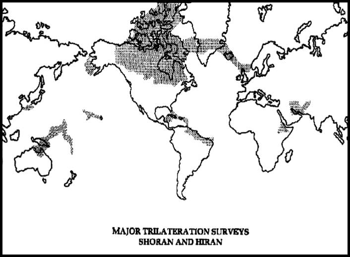
As shown in DMA Technical Report, 80-003, Geodesy for the Layman, December 1983.

HIRAN surveys aimed at keeping the number of ground stations to a minimum. Line-of-sight between the stations and the aircraft, signal reduction by intervening terrain, and the final geometric integrity of the network, all had to be considered. It was crucial that the final plan had the stations sited so that the resultant trilateration lines would intersect in a manner that would minimise errors and thus enable specified survey and map accuracies to be met.

If we can remember the world of the 1960s the places that still required detailed mapping were among the most isolated in the world. Due to line-of-sight considerations, the ground stations had to be on the highest points in these desolate areas. All in all not a simplistic set of requirements for the time!

Even more demanding were the requirements for the airborne platforms. Four Boeing RB-50 (B-29 Superfortresses with major modifications for reconnaissance purposes) were used on project AF 60-13. As quoted in The MATS Flyer of April 1964 they were required to “be at a given point under proper atmospheric conditions with the electronic equipment precisely warmed, tuned and calibrated”. Interestingly the Southwest Pacific Survey included several long lines, the longest of which (a HIRAN record) was 576 miles (930 km). The measurement of these long lines required the RB-50s to struggle to achieve at least 43,000 feet when their specified ceiling was only 37,000 feet!  

Project AF 60-13

The Project had four phases, although Phase 1 was split into Phase 1A and 1B. As Phase four focussed on surveying from the Marshall Islands down through what is now Kiribati (pronounced Kiribas) and Tuvalu to Fiji, Phases I – 111 are of main interest here.

Phase IA of Phase I was to connect sites within the Caroline Islands then a United States Trust Territory.

Phase IB of Phase I was then to connect sites in the Bismarck Archipelago, then an Australian United Trust Territory, to Phase IA.

Phase II was then to connect sites within the Marshall Islands (containing Bikini Atoll), also then a United States Trust Territory to Phase IA.

Phase III was then to connect Cape York, central Queensland and Arnhem Land sites, through PNG sites, to Phase IB.

However, for operational and diplomatic reasons (once in Australian territory they stayed until the work was completed) Phase III followed Phase IB leaving Phase II to the end.

The original plan for the Australian connections shows 11 coastal stations. However, two more central Queensland stations were occupied increasing the number of stations on the Australian 1st order network to six and thereby strengthening the resulting network.  

Phase IB AND III Trilateration Network

Phase IB and III resulted in 29 HIRAN stations being occupied (13 Australian, 9 PNG, 7 Bismarck Archipelago).

Six of the HIRAN stations were installed on stations of the Australian 1st order network to connect to that system as listed below:

No.	Station	Location
32	A468	Queensland
33	U136	Northern Territory
34	RANTYIRRITY POINT U204	Northern Territory
35	MOUNT DUNDAS U214	Northern Territory
60	BISHOP CREEK A427	Queensland
61	HILLTOP A411	Queensland

Two stations were installed in Australia on sites not tied to a ground survey system:

No.	Station	Location
30	NORMANTON	Queensland
31	EDWARD RIVER MISSION	Queensland

Five stations were installed on an extension of the tellurometer traverse through Cape York in Australia being:

No.	Station	Location
25	MOUNT SCOTT	Prince of Wales Is. Queensland
26	MOUNT TOZER B077	Queensland
27	B069	Queensland
28	MOUNT PIEBALD B065	Queensland
29	BISHOP	Queensland

Three HIRAN stations were installed on stations included in a closed loop of tellurometer traverse in PNG as follows:

No.	Station	Location
21	SUAU	PNG
22	MYOLA aka KENEVI	PNG
23	AIRD HILLS 1963	PNG

Thirteen stations were installed on sites in PNG, the Bismarck Archipelago, and other islands. As listed:

No.	Station	Location
9	LEA	MANUS ISLAND
10	NOMA	MUSSAU ISLAND
11	PILIKOS	NEW HANOVER ISLAND
12	MORU	SIMBERI ISLAND
13	TSINON	BUKA ISLAND
14	NEW TANGI	NEW BRITAIN ISLAND
15	NANDAN	NEW BRITAIN ISLAND
19	KUMUN	KARKAR ISLAND
20	NOEL	NOLEI ISLAND, LUSCANY ISLAND
24	DARU	DARU ISLAND
36	TURU	PNG
37	SEPIK HIRAN aka KAHAN	PNG
38	SUKI	PNG

The Outcome

To connect the 29 stations, 141 HIRAN distances were measured. The longest line measured was 545 miles (880km), the shortest was 84 miles (135km), and the average length was 346 miles (555km).

The USAF HIRAN connections to the traverse up Cape York placed an additional 135 points on the Australian Geodetic Datum extending it to Papua New Guinea. (DMA, 1983).  

Acknowledgements

Mr Jim Kinter Sr., Webmaster for the www.1370th.org site, is gratefully acknowledged for granting me permission to use material from that site in this paper. Also to the men who provided the material appearing on that site especially Mr Charles Alvis and Mr Terry Gust whose documents were especially helpful. Additionally Mr Ed Burke for his photo of the RB50 at Port Moresby.

References

Aerial Survey and Photomapping History, (2007). Aerial Survey and Photomapping History & Air Force Photo Mapping Association website, USA, <http://www.1370th.org>.

Boeing. (1962), RB50 Manual, Aerial Survey and Photomapping History 2007, Aerial Survey and Photomapping History & Air Force Photo Mapping Association website, USA, <http://www.1370th.org/rb50/rb50-f_manual/rb50man.htm>.

Clark, D. (1963), Plane and Geodetic Surveying for Engineers, Vol 2, 5th Edition, London, Constable & Co. Ltd. pp 308-315.

DMA. (1983), DMA Technical Report, 80-003, Geodesy for the Layman, December 1983,

< www.ngs.noaa.gov/PUBS_LIB/Geodesy4Layman/TR80003A.HTM>.

History of the 1370th Photo-Mapping Wing, 1962-64, Aerial Survey and Photomapping History 2007, Aerial Survey and Photomapping History  & Air Force Photo Mapping Association website, USA, <http://www.1370th.org/1370PMW/documents/1370docs.html>.

Rabchevsky, G.A.(Ed.), (1984), Multilingual Dictionary of Remote Sensing and Photogrammetry, American Society of Photogrammetry, Falls Church: Virginia, USA.

USAF. (1965), Special Report of Results, Australian Controlled Territory, Southwest Pacific Survey, Project AF60-13, 15 January 1965, Volume 1, Prepared by 1370th Photo-Mapping Wing, Air Photographic & Charting Service, USAF, Albany, Georgia, USA. 

RB-50 at Jackson Field, Port Moresby

MYOLA aka KENEVI from ground and Australian geodetic survey helicopter – note sighting vanes attached to HIRAN mast to aid geodetic observations from surrounding sites.