NovaSAR : Australia’s Latest Involvement with Synthetic Aperture Radar (SAR) Data

by Paul Wise, 2023

Introduction

NovaSAR 1 was launched in September 2018. This minisatellite was developed collaboratively by SSTL (Surrey Satellite Technology Ltd.) and Airbus Defence & Space Ltd, with funding from organisations in the UK, India, Australia and the Philippines. NovaSAR 1 carried new, low cost, S band SAR (Synthetic Aperture Radar) technology.

A few years earlier in 2015 the European Space Agency (ESA) released a new synthetic aperture radar dataset from the National Aeronautics and Space Administration’s (NASA) SEASAT. In 1978, only six years after the first Landsat satellite, then the Earth Resources Technology Satellite, was launched, a complementary earth observing technology, SAR, was orbited. Lasting only 106 days, before electrical problems forced its shutdown, SEASAT SAR nonetheless demonstrated that a spaceborne radar system could add to our knowledge of the Earth. ESA has now retrieved, consolidated and reprocessed the SEASAT data it held and made it publicly available.

During the 40 years between SEASAT and NovaSAR, SAR systems have been developed and launched by many countries and this article summarises those activities.

SAR from SLAR and Radar

Extensively developed during World War 2, radar, originally an acronym for RAdio Detection And Ranging, but today a word in its own right, transmits its own electromagnetic radiation thereby being an anytime, all weather system. When a transmitted radar beam strikes an object, part of the energy is reflected back to a receiver which analyses the return and in its simplistic form provides distance and direction to the object.

A two dimensional image of the terrain can be obtained by using radar to illuminate an area and record photographically or electronically the returns, or backscatter, from the many ground points illuminated. Such a system is an imaging radar.

Airborne radar in the form of SLAR (Side Looking Airborne Radar) was an imaging radar. To avoid all the return signals being received simultaneously radar imaging systems had their antennae configured to look to the side, hence side looking. The SLAR antenna emitted a fan shaped beam with the narrow side of the fan parallel to the along track direction of flight (or azimuth) of the platform. The wider side of the fan was then parallel to the cross track direction of flight (or range). Please refer to the figure below. As the SLAR moved along a flight path, the area illuminated by the radar, or footprint, was moved along the terrain in a swath, building the image. In such an image brighter areas represented high backscatter, darker areas represented low backscatter.

The use of SLAR at very high altitudes was constrained by its resolution in the along track (azimuth) direction. Azimuth resolution was directly proportional to the range of the object, the higher the SLAR the longer the range. Thus SLAR was unsuited to spaceborne operations.

SAR overcame the SLAR limitations by processing simultaneously the time delay and Doppler shift information contained in the returned signals from a point in the terrain, while that point remained illuminated by the radar beam. The resolution now became independent of range and related only to the accuracy of the measurement of the differential time delay and Doppler frequency shift. This was the equivalent of synthesising a long antenna from a much shorter physical antenna. More detail may be found at Annex A.

SAR Parameters

The emitted wavelength or frequency of a SAR system is still indicated by a World War Two radar classification system. This band system classified a range of wavelengths/frequencies as belonging to a particular band as shown in the table below (note that these values are only a guide and wavelength is inversely proportional to frequency).

BAND	WAVELENGTH	FREQUENCY
P	60 cm	0.5 GHz
L	23.5 cm	1.28 GHz
C	5.7 cm	5.3 GHz
X	3 cm	10 GHz
Ku	2 cm	15 GHz
Ka	1 cm	30 GHz

All electromagnetic energy has electric and magnetic fields operating at right angles to each other and normal to the direction of propagation. This allows the electric field vector to be polarised in either the horizontal (H) or vertical (V) plane. SAR systems as they evolved could thus be set to emit and receive in some combination of these horizontal and vertical planes. Initially emitting and receiving in the horizontal plane or HH was used and then VV, emitting and receiving in the vertical plane was tried. Today the four combinations HH, VV, HV and VH can be available. Objects in the terrain were found to reflect the emitted beam at different polarisations and some regions, notably vegetated areas, depolarised the beam.

INDICATIVE SAR PARAMETERS FOR COMMON APPLICATIONS

APPLICATION

WAVELENGTHS

INCIDENCE ANGLES

POLARISATIONS

VH/HV

Hydrology

Soil moisture

Land/water interface

Agriculture

Standing biomass

maximises path through canopy

Moisture content

minimises sub-canopy contribution

Forestry

Woody biomass

maximises penetration through canopy

Green biomass

maximises canopy sensitivity

Defoliation

maximises canopy sensitivity

Deforestation

sensitive to canopy and trunk

Geology

Desertification

Surface roughness

The incidence angle is the angle at which the radar beam strikes the terrain as measured from the normal to the surface at the point on the ground. As this angle varies across the swath illuminated by the beam, the angle is usually quoted for mid swath.

Another angle that is quoted in the look angle. The look angle is the angle of the antenna when transmitting and receiving. In early SAR missions this angle was fixed but during later missions the angle could be varied between some 20 and 40 degrees.

SAR System Summary

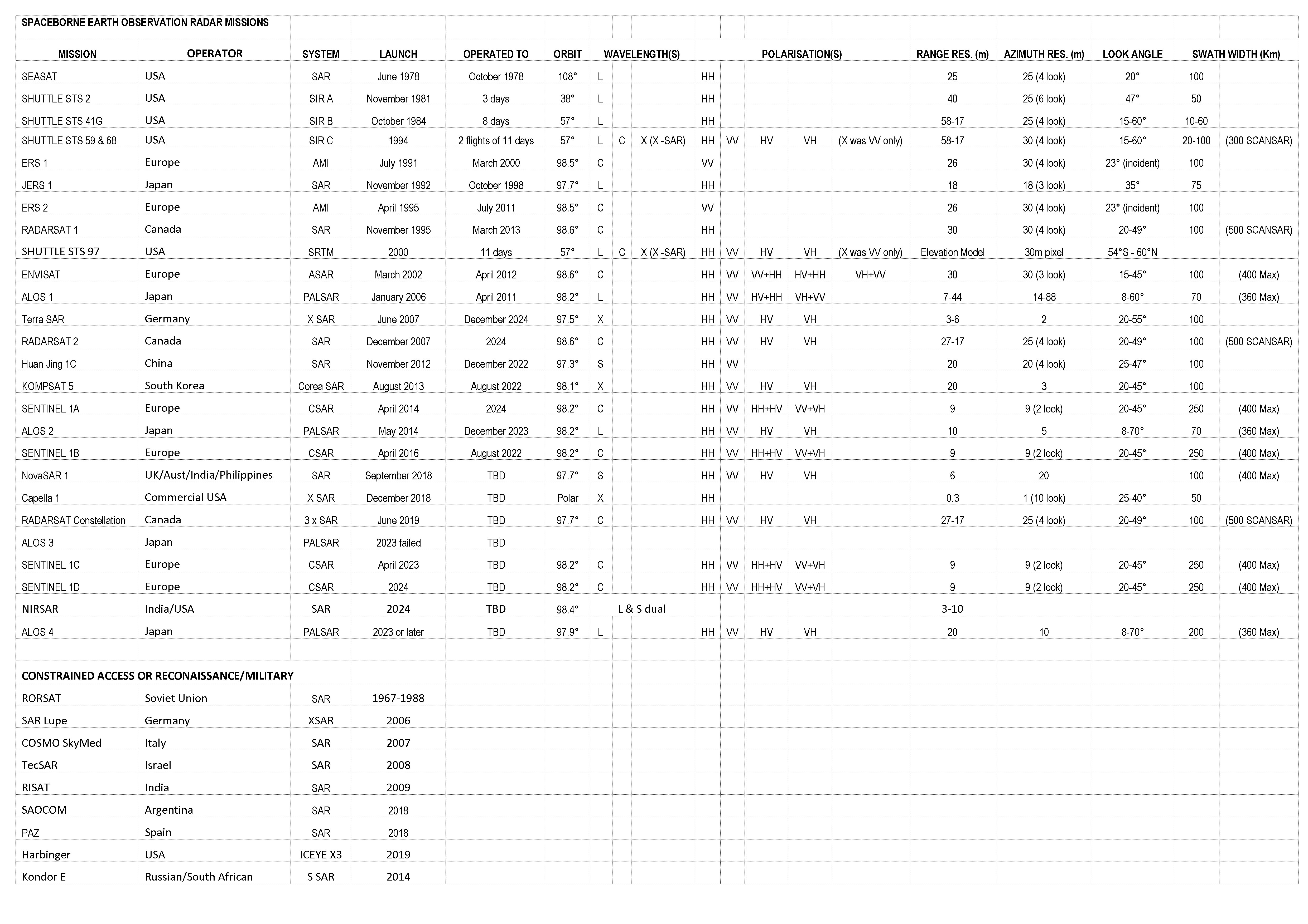
This table is a best efforts list of SAR missions and their parameters to date along with those planned for the next few years.

After the USA had terminated SEASAT’s mission their next SAR systems were orbited aboard their Shuttle. Shuttle Imaging Radar (SIR) A, B and C systems each carried improvements providing a wider range of data for evaluation of the technology.

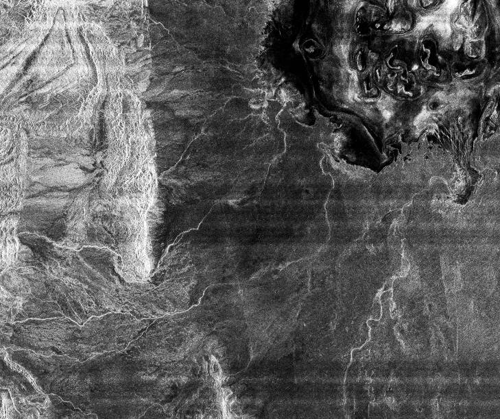
SIR A provided, what was described as an extraordinary image, in November 1981. To understand the impact of the SIR A image it is shown below combined with a Landsat view of the same terrain.

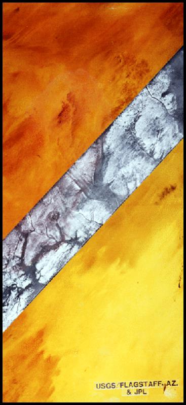
Combined LANDSAT/SIR A image of the South East Sahara Desert covering an area of some 150 by 250 kilometres

where subsurface palaeodrainage systems are visible on the radar image which are not visible on the LANDSAT image;

courtesy of NASA/JPL.

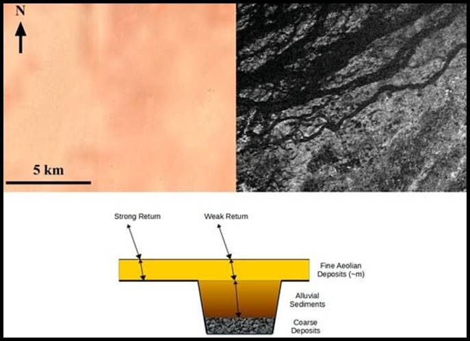
In this hyper arid region of the Selma Sand Sheet of the Sahara Desert, Sudan, the radar waves penetrated the small dry sand particles to depths of several meters or so. The channelled subsurface topography then reflected some of that energy revealing the dark (low backscatter) channel system and brighter (higher backscatter) relatively higher terrain, as depicted in the example above.

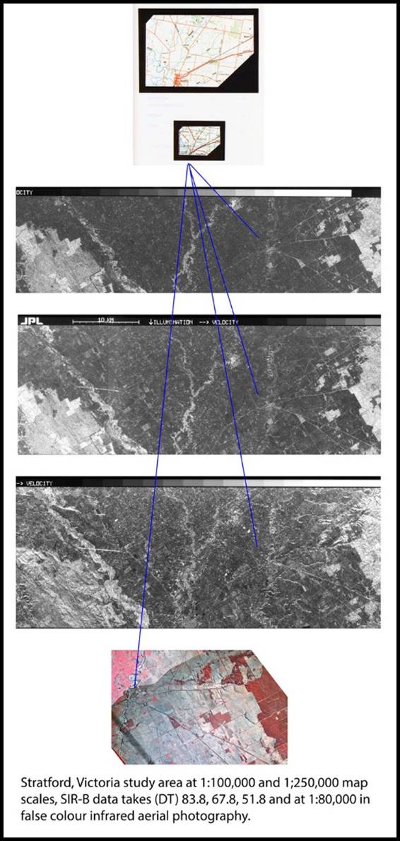
One of forty-three proposals from researchers outside the United States which was accepted, resulted in SIR B data being acquired for some specific Australian sites, during October 1984. The Australian Multi experimental Assessment of SIR B (AMAS) was the proposal of the University of New South Wales, then Centre for Remote Sensing. SIR B digital and photography imagery included the following 3 Data Takes around Stratford, Victoria. Please refer to the image below which can be viewed at full resolution via this link. Data Take (DT) 83.8 was acquired with a look angle of 48 degrees, DT 67.8 at a look angle of 37 degrees and DT 51.8 at 17 degrees. The imagery is courtesy of NASA, JPL and UNSW.

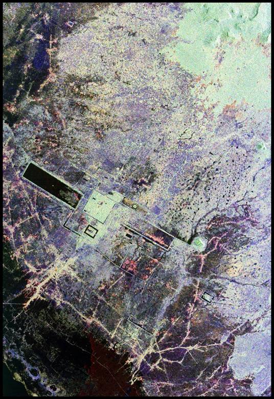
On September 30, 1994, the SIR-C/X-SAR systems penetrated the tropical environment to record data over Angkor Wat in Cambodia. Combining data from the L band (horizontally transmitted and received) as red, L band (horizontally transmitted and vertically received) as green and C-band (horizontally transmitted and vertically received) as blue the image shown below was generated revealing hitherto undiscovered/unknown archaeological detail.

SAR showed that this anytime, all weather technology was extremely sensitive to small changes in surface roughness, and was useful for assessing changes in waves, sea ice features, ocean topography and flood mapping. Later volcano monitoring and earthquake research were added to the list when a technique known as radar interferometry was developed. Using two SAR images of the same terrain taken from slightly different locations in space, differences between these images allowed the calculation of surface elevation, or change. Initially the two images came from different orbits of the same satellite but little inaccuracies in the orbital positions were reflected in the final result.

During the Shuttle Radar Topography Mission (SRTM), a specially modified radar system flew onboard Space Shuttle Endeavour for 11 days in February of 2000. To get two SAR images taken from different locations the SRTM hardware consisted of one radar antenna in the shuttle payload bay and a second radar antenna attached to the end of a mast that extended 60 meters (200 feet) from the shuttle as shown in the image below. The fixed and known separation of the antennae removed a significant variable from the interferometric process.

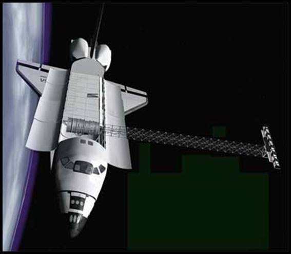
Artist representation of SRTM in space

Artist representation of SRTM in space. Main antenna is located in the payload bay, the mast is deployed to 60 meters (200 feet),

and the outboard antenna is attached to the end of the mast;
courtesy of the German Aerospace Center.

SRTM was launched into an orbit with an inclination of 57 degrees. This allowed SRTM's radars to cover most of the Earth's land surface that lies between 60 degrees north and 56 degrees south latitude, about 80 percent of Earth's land mass. The Shuttle Radar Topography Mission resulted in the international community producing digital elevation models on a near global scale to generate the most complete high resolution digital topographic database of Earth. When you consider that this model covers regions such as the equatorial jungles, remotest deserts and the roughest of terrain, where obtaining such a data model by traditional methods would have taken decades if at all, this was an extraordinary achievement.

During and since the Shuttle SAR missions the Europeans, Japanese and Canadians have been at the forefront of orbiting SAR systems, as listed below.

Europe	Launched
ERS 1	1991
ERS 2	1995
ENVISAT	2002
SENTINEL 1A	2014
SENTINEL 1B	2016
SENTINEL 1C	2023
SENTINEL 1D	for 2024
Japan
JERS 1	1992
ALOS 1	2006
ALOS 2	2014
ALOS 3 (failed0	2023
ALOS 4	2023
Canada
RADARSAT 1	1995
RADARSAT 2	2007
RADARSAT Constellation	2019
Germany
Terra SAR	2007
China
Huan Jing 1C	2012
South Korea
KOMPSAT 5	2013
ACRONYMS
ALOS (Advanced Land Observing Satellite), also known as Daichi
ENVISAT (ENVIronmental SATellite)
ERS (European Remote sensing Satellite)
JERS (Japanese Earth Resources Satellite)
KOMPSAT (KOrean Multi Purpose SATellite)

In 2018, Capella Space, a commercial American space company contracted to American government agencies, launched an X SAR on Capella 1. This is the first of a block of seven mini SAR satellites. Meanwhile NASA and the Indian Space Research Organisation (ISRO) are collaborating on NISAR (NASA-ISRO Synthetic Aperture Radar satellite) planned for a 2024 launch.

Australian Support for Earlier SAR Missions

During the 1980s and 1990s Australia was heavily involved with initially upgrading facilities and then operationally downlinking, processing and archiving SAR data from primarily ERS 1, JERS 1, and RADARSAT 1.

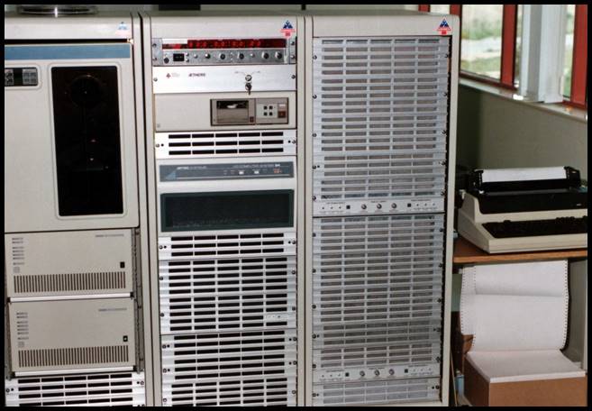
The then British Aerospace Australia (BAeA) AETHERS Fast Delivery Processor at ACRES in 1992.

The AETHERS (Australian Equipment To Help [process] ERS) Fast Delivery Processor (FDP) was proposed by CSIRO to support the large number of Australian scientists who had been accepted as investigators on the European Space Agency satellite ERS 1 SAR experiment. The FDP was to deliver preliminary images at 1/10th real time, be a world leader and surpasses anything available in Europe at the time.

Landsat Thematic Mapper and ERS 1 SAR image over a region around Lake Eyre, Australia.

The FDP was delivered in November 1992 with its development funded by the then Australian Space Office. The hardware was to be based on low cost, custom made, vector processors attached to commercial computing equipment and a continuous processing algorithm. In its initial configuration the FDP was to be used to process images from the ERS 1 SAR, delivering full scene (100km x 100km) products.

NovaSAR

NovaSAR 1 was launched in September 2018. The launch vehicle was provided by ISRO and took place from SDSC (Satish Dhawan Space Center, formerly Sriharikota Range or SHAR), ISRO's launch centre on the south east coast of India, Sriharikota. The launch provider was Antrix Corporation Ltd, the commercial arm of ISRO.

This minisatellite was developed collaboratively by SSTL (Surrey Satellite Technology Ltd, a wholly owned subsidiary of Airbus) and Airbus Defence & Space Ltd, with funding from organisations in the UK, India, Australia and the Philippines. NovaSAR 1 carried new low cost S band SAR (Synthetic Aperture Radar) technology. A constellation of three satellites for more frequent revisit times is planned but with now only one satellite the revisit time is 16 days.

The S SAR instrument was derived from Astrium’s airborne radar technologies. Access to this technology came about when Airbus Defence & Space became a division of the Airbus Group after the European Aeronautic Defence and Space Company (EADS) was reorganised. This reorganisation had followed Astrium, then an aerospace manufacturer subsidiary of the European Aeronautic Defence and Space Company, being merged with Cassidian, the defence division of EADS. Please refer to Astrium, Cassidian and EADS Evolution into Airbus and its Relationship with SSTL, SPOT and ESA, at Annex B , for details.

In 2003 it was reported that EADS Astrium has successfully developed an Airborne Synthetic Aperture Radar (SAR), called the MicroSAR Airborne Demonstrator, which could be applied to both spaceborne and airborne SAR systems, including the spaceborne MicroSAR system and the airborne QuaSAR system. This technology was then claimed to be a major breakthrough in low cost SAR systems. Funded by the then British National Space Centre (BNSC), an agency of the Government of the United Kingdom organised in 1985, that coordinated civil space activities for the United Kingdom, it was replaced in 2010 by the UK Space Agency.

The MicroSAR Airborne Demonstrator had completed a series of successful trials mounted on a Defence Science and Technology Laboratory (DSTL), UK, Britten-Norman Islander aircraft. Operating between 3000 and 7000 feet over Portsmouth and the surrounding area, the trials generated high quality X-band imagery through cloud. The Airborne Demonstrator instrument, which was only 75 centimetres high and weighed only 49 kilograms, was able to provide image resolution down to 1metre, both day and night, and in all weather conditions. At the heart of the instrument was the generic CORE Radar Central Electronics developed by EADS Astrium. This could be adapted to a wide range of radar frequencies and was suitable for both space and airborne platforms, including UAVs. A C band system was currently being built by EADS Astrium for the Canadian SAR satellite, Radarsat 2. In addition to the central electronics, the airborne demonstrator included an innovative, very low cost, active phased array antenna and an inertial measurement unit to measure and record the aircraft motion, thus allowing motion compensation in the image processing.

Specifically designed for low cost programmes and optimised for shared launch opportunities, the NovaSAR S SAR has four operational modes: ScanSAR, Maritime Surveillance, Stripmap and ScanSAR Wide. The ScanSAR mode covers a swath width of 50-100 kilometres at a spatial resolution of 20 metres, whilst the ScanSAR Wide mode offers a larger swath width of 100-50 kilometres at a resolution of 30 metres. The Stripmap mode has the finest resolution at 6 metres, covering a swath width of 15-20 kilometres. The final mode, Maritime mode, is an experimental mode used for the detection of ships in the open ocean. At a medium resolution of 30 metres, the large swath width of up to 750 kilometres enables effective ship detection via azimuth ScanSAR imaging.

Operational impression of NovaSAR 1; courtesy SSTL.

Before the launch in 2017, SSTL signed an agreement to provide Australia’s CSIRO (Commonwealth Scientific and Industrial Research Organisation) a 10% share of the tasking and data acquisition capabilities from NovaSAR. Post launch in 2019, a similar agreement was signed with the Republic of the Philippines’ Department of Science and Technology - Advanced Science and Technology Institute (DOST-ASTI).

The agreement gave CSIRO tasking priorities and the ability to access the raw data directly from the satellite, and a license to use and share the data with other Australian companies and organizations over an initial 7 year period. In 2021 it was announced that Australian researchers could apply to direct NovaSAR 1 by accessing Australia’s share of the satellite, managed by CSIRO. This marked the first time Australia had managed its own source of Earth observation data.

NovaSAR 1 coverage of the Australian region at July 2021.

NovaSAR 1 data is downloaded to a receiving station near Alice Springs owned by the Centre for Appropriate Technology (CfAT), Australia’s first and only Aboriginal owned and operated ground segment service provider.

The CSIRO, Centre for Earth Observation controls all facets of NovaSAR in Australia and the imagery received has enabled a complete mosaic of Australia to be assembled.

NovaSAR Data in Use

A brief search of the internet revealed three articles mentioning the use of NovaSAR’s data. A 2022 paper by Levin and Phinn, Assessing the 2022 Flood Impacts in Queensland Combining Daytime and Nighttime Optical and Imaging Radar Data, reported the use of Capella and NovaSAR data over Brisbane. A University of New South Wales led project, Quantifying the Past and Current Major Australian Floods with SAR and Other Satellites, aims to develop and operationalise smart analysis of SAR and optical satellite imagery (primarily NovaSAR and Sentinel missions) to address time critical applications such as flood mapping…. A 2021paper by Parker, Castellazzi, Fuhrmann, Garthwaite and Featherstone, Applications of Satellite Radar Imagery for Hazard Monitoring : Insights from Australia states that future opportunities to improve national hazard identification will arise from new SAR sensing capabilities, which for Australia includes a first ever civilian EO capability, NovaSAR 1.

Annex A

A REVIEW OF SYNTHETIC APERTURE RADAR IMAGING

Introduction

To simplify this topic as much as possible it was necessary to state some aspects of theory without proof and minimise the derivation of mathematical equations. For most users such an in depth of understanding is not required.

Basic Principles of Radar

Radar is an active (in that it generates its own radiation) remote sensing system that has four basic components :

1. transmitter

2. antenna

3. receiver

4. recording device

Figure 1: Typical SAR geometry

The microwave energy which is generated by the transmitter, in pulses or bursts, is directed at the ground by the antenna. To avoid all the return signals being received simultaneously radar imaging systems have their antenna configured to look to the side, hence the original name Side-Looking Airborne Radar (SLAR). Refer to Figure 1. The terrain scatters this incident radiation, some of which is reflected back to the antenna. Subsequent processing of the return signal allows particular characteristics to be extracted and compared (correlated) with a delayed replica of the transmitted signal. The magnitude of the delay is today, recorded digitally.

Real Aperture Radar

Side Looking Airborne Radar (SLAR) or brute force radar are examples of real aperture radar which use antenna beamwidth to control azimuth resolution and pulse duration to control range resolution.

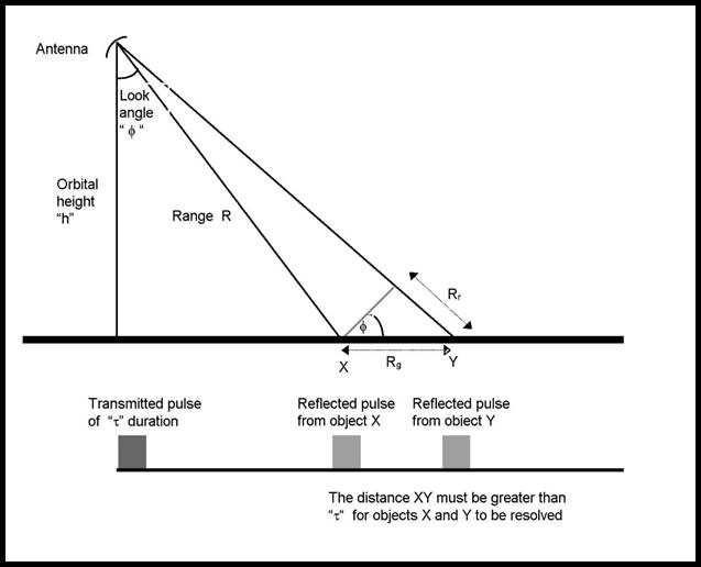
Figure 2: The relationship between range and ground resolution.

The azimuth resolution of real aperture radar R_a is given by:

R_a= b * R (1)

where b is the azimuthal beamwidth of the antenna (radians); and

R the slant range from the antenna to the ground.

(Note that the slant range will vary across the swath)

The beamwidth of the antenna b is related to its physical length and to the wavelength of the emitted radiation in the following way:

b (radians ) = l / l (2)

where l is the wavelength of the emitted radiation, and

l is the physical length of the antenna;

and R is related to the height h of the antenna platform and its look angle f giving:

R_a = b * R = (l / l) * (h / cos f) (3)

Using any practical figures it can be seen that at satellite orbital height the azimuthal resolution obtained by such a system is clearly unacceptable.

In the range direction range resolution R_r is given by:

R_r = c * t / 2 (4)

where c is the velocity of electromagnetic radiation, and

t is the pulse duration.

It can be seen in Figure 2 that two objects in range can only be resolved if their echoes are separated by at least the pulse duration when received by the antenna.

The distance R_r is not in the horizontal (ground) plane but can be converted to a horizontal distance R_g using the look angle f as shown in Figure 2. Thus

R_g = c * t / (2*sin f) (5)

As there are real electronic engineering limits to reducing the pulse duration using any practical figures it can be seen that the ground range resolution obtained by such a system is again unacceptable. SAR systems were therefore a logical development using pulse width and a synthetic antenna to improve spatial resolution at satellite orbital heights.

Synthetic Aperture Radar (SAR)

The higher spatial resolution of SAR systems is based on correlating the received terrain echoes with the transmitted signal producing a short pulse where the energy of the received signal is compressed.

The SAR transmitted signal is not a simple pulse but a linear chirped waveform or ranging chirp, where the frequency increases linearly with time. After correlation, the short pulse produced has an effective width inversely proportional to the chirp bandwidth B.

In equation 5 the pulse duration t can now be replaced by the compressed pulse duration 1/B which will define the ground range resolution of a SAR system. Thus:

R_g = c / (2B*sin f) (6)

In azimuth the chirp is induced by the motion of the antenna platform as it approaches and recedes from the object. This increase and decrease in frequency are the classic Doppler effect and the frequency variation over time is close enough to be accepted as linear.

The azimuth chirp, after correlation with a replica of itself (the azimuth chirp is affected by earth rotation and platform attitude changes requiring the replica be derived from the return signal), produces a short pulse with an effective width, in time, equal to the reciprocal of the Doppler bandwidth B and chirp length T (1/ BT). The width of this pulse determines azimuth resolution as follows.

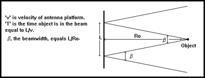
Figure 3: Azimuth geometry of an object in the radar beam.

From Figure 3 any range R can be computed from an initial range R_o, and the motion of the antenna platform. That is

R = Ö[R_o² + (vT)²] as L = vT (7)

As the term (vT)² is small compared to R_o² we can apply a series expansion with sufficient precision to yield:

R » R_o + v²T² /2R_o(8)

That is the one way change in range, can be equated to a change in phase of v²T² /2R_o. Converting this change of phase to a two way change in radian measure results in the following:

j = 2p v²T² / lR_o(9)

The above shows that it is possible to predict or precompute the phase of the returned signal from a specific ground point. This in turn allows us to phase correct the return signal allowing us to use a longer data length from the ground point. This technique is called focusing.

We can now find the corresponding frequency change as frequency is the first differential of phase thus:

¶j/¶T = w = 2pf = 4p v²T/ lR_o(w is angular frequency, f is frequency) (10)

resulting in:

f = 2v²T/ lR_o(11)

giving the Doppler bandwidth, b, for the time period T as:

b = 2v²/ lR_o(12)

The chirp length is equal to the time that the object is in the beam, refer Figure 3, which is calculated by dividing the distance travelled by the antenna while the object was in the beam divided by the velocity of the platform:

T = L / v (13)

Also we have the following relationship from equation 2 and Figure 3:

b = l / l = L / R_o or L = l R_o / l (14)

which gives after substitution in equation 13:

T = l R_o / v l (15)

Manipulating equations (12) and (15) we get:

1/ B T = l / 2v seconds of time (16)

which at velocity, v, equates to a ground distance of l/2 where l is the physical length of the antenna. It needs to be noted that only under focused conditions is the theoretical resolution in azimuth equal to half the physical antenna length.

Using ERS data where B = 15.5MHz, f = 23° at mid-swath and the physical length of the ERS antenna is 10m we can calculate:

R_g = 24.7m (mid-swath) and

R_a = 5m for single look and 15m for three looks.

These are theoretical figures but compare well to ERS actual figures of ground range resolution equal to 22m to 28m across the swath (resampled to 20m) and a best single look azimuth resolution of 6.5m and three look azimuth resolution of 16.8m.

You will note that, before final resampling to a fixed square pixel size, a single look product pixel would have a rectangular dimension of 20m by 5m in range and azimuth respectively whereas the three look product the pixel dimension is approximately square (20m x 17m). As well as reducing noise (Radar Speckle) look extraction helps to generate approximately square pixels before final resampling to the output pixel size.

The above shows that the spatial resolution for SAR systems is independent of platform height and distance to objects and is essentially a function of transmitted chirp characteristics and physical antenna length. However, the limits of SAR spatial resolution are constrained because radar complexity, storage and processor requirements all increase with increasing range and wavelength, and power handling considerations increase sharply as the antenna length is reduced.

SAR Processing

From a given transmitted chirp the set of return chirps from the terrain form a range line of data. As the return chirps are a continuous signal this signal is sampled (range gated) and these samples are stored on magnetic tape. Subsequently this data is transferred to computer memory for processing. The complete set of radar reflections for a given area of terrain will therefore consist of many range lines.

Radar returns from a point target in the terrain will occupy a number of computer memory cells (range bins) in each range line and a number of memory cells in azimuth (azimuth bins). Range and azimuth correlation takes this spread of data and compresses it to a single bin corresponding to the return from the point target.

This procedure implies that the slant range to a point target is constant irrespective of the position of the platform. In practice, the slant range varies quadratically as a function of the distance between the platform and the point directly abeam the object. During data acquisition earth rotation causes a skew effect and together with the continuous slant range variation leads to the range compressed lines of data being curved in the memory ie. the data for the point target migrates across range bins as a function of azimuth. This causes errors following azimuth compression unless this Range Cell Migration or Range Walk is corrected. Range Cell Migration is corrected following range compression and before azimuth compression.

Figure 4 shows the formation of an image after the data is first corrected for Range Cell Migration and compressed so that the energy from a single point on the ground is stored as a single point in the processor memory.

Instead of compressing the entire azimuth signal energy in one operation the Doppler spectrum may be divided into several segments or looks; this process is called look extraction and can be considered similar to viewing the same object from several different viewpoints. A single image cell is then formed by summing the intensity of a number of looks. Processing by look extraction has the advantage of removing some of the speckle inherent in coherent imaging systems. It also has the disadvantage however of reducing the azimuth resolution from the theoretical one look value of l/2 to a value equal to the product of the number of looks and l/2.

Radar Speckle

Due to the monochromatic and coherent nature of the microwave radiation, the return signal is the vector addition of signals resulting from reinforcement or negation from different picture elements within the resolution cell. This creates the speckle effect on SAR imagery which appears as a grainy, granular noisy phenomena of black and white random pixels. As speckle behaves like multiplicative noise the effect may be so severe as to make an image uninterpretable without significant filtering or look extraction. It also introduces large uncertainties in the determination of radar backscatter intensity.

Speckle may be reduced in two ways. By look extraction as discussed above or by filtering single look images. If look extraction is used, and it is currently the most common method, the reduction in the noise is proportional to the reciprocal of square root of the number of looks (1/Öno. of looks). For example, a four look image has the noise halved (1/Ö4 = 1/2).

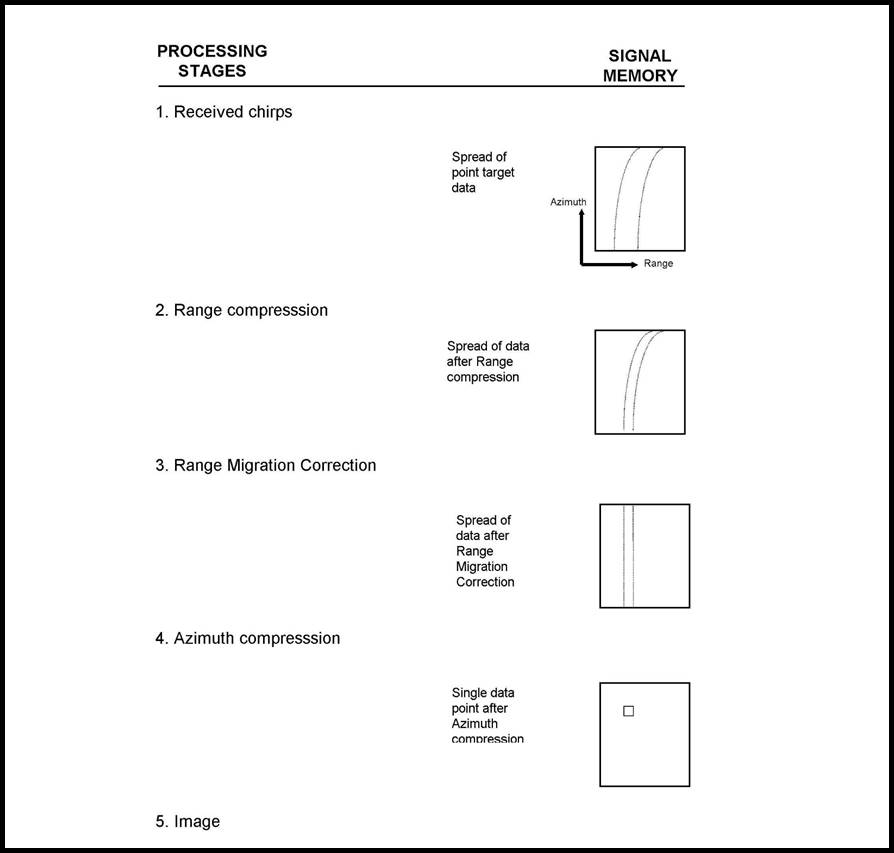
Figure 4: Major stages in the processing of SAR data.

Relief Distortions in SAR Imagery

The geometry of radar imagery is fundamentally different from both aerial photography and scanner imagery as radar is a distance rather than an angle measuring system. Radar images are therefore range projections and the features imaged and their positions are distorted. The distortion is essentially a function of both the data recording and processing system, the platform and shape of the earth.

Ground range nonlinearity caused by the variation in the look angle across the swath, skew and a second order effect caused by a variation in the rotational velocity of the earth between near and far range are all substantially eliminated during processing. Distortions caused by relief, however, remain.

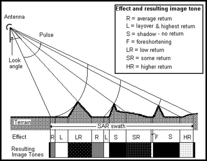
Figure 5: Relief distortions and resulting image tones from the interaction of the radar beam with the terrain (adapted from Lillesand & Kiefer).

Where two points in the terrain having different elevations have identical slant ranges they will both be projected into the same point on the radar image. If the top of an object has a shorter range than its base the top will be recorded away from its true plan position in the range direction, towards the sensor. This effect is called layover. Geometrically, for layover to occur the angle of slope of the terrain must be greater than the radar look angle. If the angle of a terrain slope facing the radar is equal to or less than the radar look angle then the slope will be foreshortened while slopes facing away will appear to be elongated. Refer Figure 5.

Where higher terrain blocks the radar beam from reaching lower terrain that region is in radar shadow.

While the layover and foreshortening effects can be removed terrain in radar shadow cannot be recovered. Users, however, need to realise that the pixels used to correct for layover are existing pixels which are just replicated and may not represent the surface imaged. For example, in a single line of data where the side of a hill is compressed to one pixel, whereas in its corrected position its length is three pixels the system can only replicate the single true pixel twice to make the two new pixels required. It cannot reimage the side of the hill.

Radar Backscatter

The grey tones in a radar image are determined by the amount of reflected radiation (backscatter) received by the system. Backscatter conveys not only the position of objects but information about their size, shape, configuration and electrical properties of the surface and sub-surface.

The average backscatter s^o (usually measured in dB, decibels) is the measure used to quantify the backscatter intensity for a homogeneous area larger than the antenna beam so as to average out the inherent noise.

The relationship of all the factors affecting the average backscatter s^o can be expressed as follows:

s^o = f ( l, P, f, a, q, e, G₁, G₂, V)

where the system parameters are:

l the wavelength of the radiation,

P the polarization of the system,

f the look angle,

a the azimuth angle, and

the scene parameters are:

q the aspect angle,

e the complex dielectric constant,

G₁ the surface roughness,

G₂ the sub-surface reflectance,

V the complex volume scatterer.

Changing one or several of these parameters will alter the backscatter and result in different information being acquired. For a given system the carrier frequency of the radar pulse is set by the system electronics so the wavelength remains fixed. Additionally the azimuth angle for a particular orbiting system relative to ground features also remains constant.

The depression and aspect angles are inter related. The depression angle determines how the radar beam strikes the terrain relative to the true vertical whereas the aspect angle determines the local vertical. Thus the combination of depression angle and the aspect angle will indicate how a particular ground surface is oriented to the beam. Radar backscatter is maximised when the sum of the depression and aspect angle is 90 degrees, ie. the ground surface is normal to the beam.

For a given system the terrain being imaged supplies the major variables of complex dielectric constant, polarization, surface roughness and volume scattering and their effect is summarised below.

Dielectric Constant

The dielectric constant of a media is a strong function of its moisture content. Moisture, and to a certain extent the salinity of that moisture, in a media can significantly increase radar reflectivity and thus reduce penetration. Depth penetration is defined as the depth below the surface at which the magnitude of the power of transmission is equal to 1/e (e = 2.718, the exponential constant) of the power just beneath the surface. The high dielectric constant of water means that even a low soil moisture content will result in little penetration and reduced backscatter.

Polarization.

Theory attributes depolarization to multiple reflections at the surface as depolarization effects have been observed to be much stronger from vegetation, comprising many reflectors in the form of leaves twigs and branches, than from bare ground.

Surface Roughness.

The roughness of the surface relative to the wavelength is the major contributor to surface scattering. Radiation striking a surface is either reflected specularly (if the surface is smooth) or diffusely (if the surface is rough). The boundary between these two extremes is a function of three parameters:

- the height of the irregularities in the surface,

- the periodic nature of the irregularity, and

- the grazing angle of the incident ray,

(ie. the angle between the incident ray and the surface).

Rayleigh's criterion relates these factors as follows:

h £ l /(8 * sin G)

where h is the height of irregularity,

l is the wavelength of the radiation, and

G is the grazing angle.

This criterion says that a surface can be considered rough if the RMS of height variations exceeds the quotient of the wavelength and eight times the sine of the grazing angle.

In general the relationship between wavelength and height variation can be considered in terms of their relative dimensions. If the emitted wavelength is smaller than the height variation then the radiation will be scattered by the terrain. If the wavelength is larger than the height variation then a greater proportion of the radiation will be reflected specularly by the terrain.

Volume Scattering.

Spatial inhomogeneities at scales relative to the radar wavelength create a volume of scatterers. Vegetation can appear as a random volume of scattering facets whereas different layers of material in the soil may also create a volume of scattering elements beneath the surface. In dealing with natural targets, the combination of vegetation, soil surface and soil profile all contribute to the complexity of the target and form part of the total surface roughness.

High Backscattering Mechanisms.

Long linear, flat or rounded metallic objects can lead to a high backscatter especially if normal to the radar beam. Corner reflectors create a higher return by reflecting a relatively greater proportion of the incident radiation back to the receiver. A corner reflector is created by either two or three planes being mutually perpendicular and as corner reflectors are generally man made they predominate in city and urban areas. Elements which have either a high dielectric constant or a length half the wavelength of the incident radiation can act as antennae. This antenna effect directs a high level of the incident radiation back to the radar antenna.

Backscatter and Tonal Differences

Bright tones in a radar image are caused by high backscatter and darker tones by low backscatter.

It should be noted that heavily vegetated and open country on a radar image have the reverse appearance to that on a black and white, passively sensed, aerial image. Compared with forests open country is a relatively high reflector of visible light and hence appears relatively bright on an aerial image. The radar wavelength generally sees open country as a smooth surface thus the majority of the radar radiation (which strikes the terrain at an angle) is reflected away from the sensor. The resultant backscatter is therefore low giving open country on a radar image a dark appearance. Conversely a forest area scatters radar radiation and relatively more backscatter is received by the sensor and hence it appears bright on the radar image. On a passively sensed aerial image forest areas appear dark. Furthermore, relief causes slopes facing the radar radiation to reflect a greater amount of radiation thus these slopes appear bright on the radar image. Terrain that slopes away from the radar can be in shadow, or reflect a reduced amount of radiation, appearing darker on the image.

A special effect of radar is noticeable in built up areas. The rectangular planes of roads and buildings strongly return the radar beam, whereas streets parallel to the beam reflect the radiation away. The high and low backscatter produces a pronounced speckle effect. Orientation of objects to the radar beam changes the pattern of backscatter and therefore the appearance of those objects in the image. Features which alter their orientation relative to the beam such as rivers and roads also alter their detectability. Streets having a particular orientation may be easily visible whilst those streets running at right angles may not be detectable. Metallic objects (particularly wire fences or power lines) that are normal to the radar beam can saturate the return and appear as very bright lines on the image.

Radar Texture

Synthetic aperture radar images contain only tonal and textural features. Texture can be considered to have three components micro, meso, and macro. Micro image texture tends to be random while meso and macro texture are spatially organised. All smooth surfaces will generally exhibit micro (fine) texture. Meso texture is produced by spatial irregularities of the order of several resolution cells. It is most striking where there is a sharp change in the relative relief of the forest canopy, or where a highly variegated soil vegetation pattern exists in a marshy environment. Macro image texture permits identification and delineation of bounded homogeneous unit areas.

Overall the interpretation of radar imagery requires that users learn a new set of rules.

SAR Interferometry

The same point in the terrain will be at a different ranges from two separated SAR antennae. In theory the two antennae can be carried by the same or separate platforms or even the same platform at a different time. However, it is preferable to avoid terrain changes between the passes.

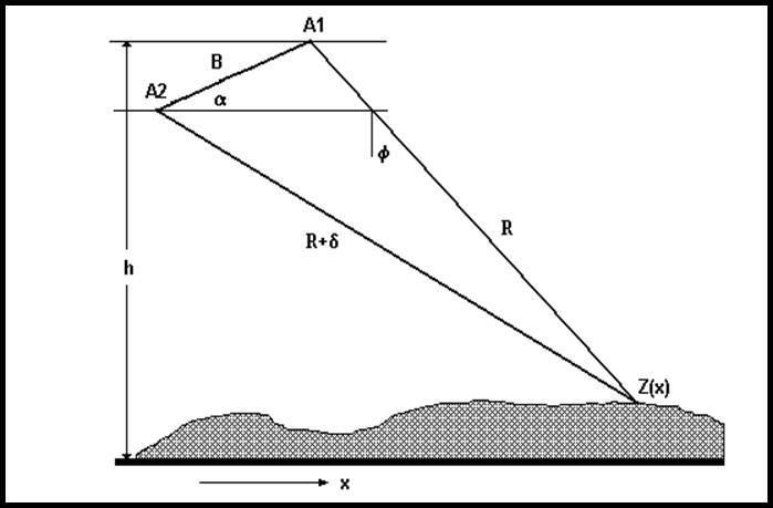
A1 and A2	the position of two SAR antennae
B	the baseline or distance separating the two antennae
H	platform altitude
Z(x)	height of the terrain
a	baseline angle
f	look angle
d	difference in range
R	Range

Figure 5: The geometry of interferometry; the use/combination of two SAR antennae to obtain height information from the terrain (adapted from Werner).

The difference in range will be indicated by a difference in the phase of the returning SAR signal. Knowing the wavelength (l) and height (h) of the particular SAR system and measuring the range (R) and phase difference (j) for points in the terrain their heights can be calculated. Refer Figure 5.

The equations involved in this process are:

d = jl / 2p (21)

sin(a-f) = [(R+d)² - R² - B²) / 2RB] (22)

Z(x) = h - R cos f (23)

In practice the derivation of terrain height is a far more complex process but over small areas with extensive ground control height accuracies of a few centimetres have been obtained.

Summary

This paper provided an overview of SAR from acquisition through processing to the interpretation of the final image and includes useful information on SAR resolution and its determination and a brief discussion of SAR backscatter determination, imagery interpretation and interferometry.

Selected Glossary

Across track: See Range.

Along track : See Azimuth.

Azimuth: The direction parallel to the ground track of the platform; also known as the along track direction.

Bandwidth: The number of cycles per second between the limits of a frequency band.

Beamwidth: The angle in degrees subtended at the antenna by arbitrary power-level points across the axis of the beam. It is approximately related to the wavelength of the emitted radiation divided by the physical antenna length.

Brute-force Radar: A radar imaging system employing a long physical antenna to achieve a narrow beamwidth for improved resolution.

Chirp: A technique to expand narrow pulses to wide pulses for transmission and compress wide received pulses to the original narrow pulse width and wave shape, to achieve reduction in required peak power without degradation to range resolution and range discrimination.

Doppler effect: A change in the observed frequency of electromagnetic radiation or other waves caused by the relative motion between the source and the observer.

Foreshortening: The compressing of the length of the slope of the terrain when the angle of that slope is less than the look angle. A slope will have no length if that slope has the same look angle as the SAR system.

Interferometry: The process of using SAR data, acquired from two separated antennae, to derive terrain height.

Layover: Displacement of the top of an elevated feature with respect to its base on the radar image.

Look angle: The direction in which the antenna is pointing when transmitting and receiving.

Looks: Obtaining a view of a feature from more than one direction to minimise fading effects of terrain.

Pulse: A short burst of electromagnetic radiation transmitted by the radar system.

Radar shadow: A no-return area extending in range from an object which is elevated above its surroundings. The object cuts off the radar beam, casting a shadow and preventing illumination of the shadowed area behind it.

Range: The distance from the radar to a target; also known as slant range.

Range Cell Migration: Where the point target undergoes a migration across range cells as a function of azimuth due to the variation of instantaneous slant range with respect to range cell separation.

Real Aperture Radar: See Brute-force Radar.

Slant range: See range.

Synthetic Aperture Radar (SAR): A radar in which a synthetically long apparent or effective aperture is constructed by integrating multiple returns from the same ground cell, taking advantage of the Doppler effect to produce a phase history tape that may be digitally processed to reproduce an image.

Selected References

Fuk-Kwok, L., Croft, C., and Held, D.N. 1983. Comparison of Several Techniques to Obtain Multiple-Look SAR Imagery. IEEE Transactions on Geoscience and Remote Sensing. Vol. GE21, No. 3, 370-375.

Laur, H. 1992. Derivation of Backscattering Coefficient s° in ERS-1.SAR.PRI Products. ESA ESRIN.

Laur, H., Meadows, P., Sanchez, J., and Dwyer, E. 1992. ERS-1.SAR Radiometric Calibration. ESA ESRIN.

Lillesand, T.M. and Kiefer, R.W. 1979. Remote Sensing and Image Interpretation. John Wiley and Sons, Inc : New York.

Rabchevsky, G.A.(Ed.). 1984. Multilingual Dictionary of Remote Sensing and Photogrammetry. American Society of Photogrammetry, Falls Church: Virginia, USA.

Raney, R.K. 1982. Processing Synthetic Aperture Radar Data. International Journal of Remote Sensing. Vol. 3, No. 3, 243-257.

Tomiyasu, K. 1978. Tutorial Review of Synthetic Aperture Radar (SAR) with Application to Imagery of the Ocean Surface Proceedings of the IEEE. Vol. 66, No. 5, 563-583.

Werner, C. 1992. Techniques and Applications of ERS-1 INSAR. Proceedings of the 1st Workshop of the SAR Interferometry Working Group. ESA ESRIN.

Wise, P.J. 1989. Spaceborne Radar Imagery - Its Acquisition, Processing and Cartographic Applications. Cartography. Vol. 18, No. 1, 9-20.

Annex B

Astrium, Cassidian and EADS Evolution into Airbus and its Relationship with SSTL, SPOT and ESA

Background

The NovaSAR S SAR instrument was derived from Astrium’s airborne radar technologies. Access to this technology came about when Airbus Defence & Space became a division of the Airbus Group after the European Aeronautic Defence and Space Company (EADS) was reorganised. This reorganisation had followed Astrium, then an aerospace manufacturer subsidiary of the European Aeronautic Defence and Space Company, being merged with Cassidian, the defence division of EADS.

European Aeronautic Defence and Space Company (EADS)

The European Aeronautic Defence and Space Company (EADS) was a major European aerospace company that built commercial and military aircraft, space systems, propulsion systems, missiles, and other defense products. It was formed in 2000 from the merger of three leading European aerospace firms : Aerospatiale Matra of France, DaimlerChrysler Aerospace (DASA) of Germany, and Construcciones Aeronáuticas S.A. (CASA) of Spain. At this time EADS owned 80% of Airbus Industrie GIE. The Airbus Industrie GIE consortium had been formed back in 1970. In 2001, Airbus Industrie GIE was reorganised as Airbus SAS (GIE for Groupement d’Intérêt Economique or Grouping of Mutual Economic Interest was a unique form of partnership instituted in French law in 1967; SAS is for Société par Actions Simplifiée or Simplified Joint-stock Company a French type of business entity, SE is for Societas Europea or European Company, a type of public limited liability company that allows you to run your business in different European countries using a single set of rules).

In 2003 EADS had acquired BAE's share in Astrium, the satellite and space system manufacturer, to become the sole owner. This was followed in 2006, by EADS acquiring BAE's remaining share in Airbus. British Aerospace (BAe) had been formed as a statutory corporation in 1977. The company brought together the British Aircraft Corporation, Hawker Siddeley Aviation, Hawker Siddeley Dynamics and Scottish Aviation. In 1986, British Aerospace became a lead partner in Eurofighter GmbH along with Alenia Aeronautica, DaimlerChrysler Aerospace (DASA) and Construcciones Aeronáuticas S.A. (CASA). In 1999, British Aerospace had merged with Marconi Electronic Systems (MES) to form BAE Systems.

EADS Defence & Security Systems had also been founded in 2003. In it, the activities of missile systems (LFK-Lenkflugkörpersysteme GmbH), defence electronics, military aircraft and telecommunications of the EADS Group were merged. The company name was changed to Cassidian, in 2010, an amalgamation of the Latin words Cassida (helmet) and meridian and focused on worldwide protection and security.

Airbus

Airbus Defence and Space was formed in 2013 as a result of the merger of Astrium, Cassidian, and the Airbus Military divisions of European Aeronautic Defence and Space Company (EADS) which was itself reorganized as Airbus. On 1 January 2014, the parent company EADS was restructured as Airbus, comprising three subsidiary companies that include Airbus Defence and Space, Airbus, and Airbus Helicopters.

Structural evolution of Airbus SE
Dec 1970	Jan 1992	July 2000	Sep 2000	Jan 2001	Dec 2006	Apr 2009	Sep 2010	Jan 2014	May 2015	Jan 2017	Apr 2017
		European Aeronautic Defence and Space Company NV						Airbus Group NV	Airbus Group SE		Airbus SE
Airbus Industrie GIE				Airbus SAS
						Airbus Military SAS		Airbus Defence and Space SAS
		EADS Defence and Security					Cassidian SAS
		Astrium SAS			EADS Astrium SAS
	Eurocopter SA		Eurocopter SAS					Airbus Helicopters SAS

Diagrammatic explanation of Astrium, Cassidian and EADS evolution into Airbus; courtesy https://en.wikipedia.org/wiki/Airbus_Defence_and_Space

Surrey Satellite Technology Ltd (SSTL)

Surrey Satellite Technology Ltd (SSTL) emerged from an experiment by a group of researchers working at the University of Surrey, to create a satellite using commercial off the shelf (COTS) components. Their home made satellite UoSat 1, was launched in 1981 with the help of NASA. UoSAT 1 was the first modern reprogrammable small satellite and was a great success, outliving its planned three year life by more than five years. Most importantly, it showed that relatively small and inexpensive micro satellites could be built rapidly to perform successful and sophisticated missions. In 1985 Surrey Satellite Technology Ltd was formed to transfer the results of the research into a commercial enterprise. In 2009 Airbus bought the majority shareholding from the University of Surrey and today SSTL is a wholly owned subsidiary of Airbus.

SPOT

The French SPOT (Satellite pour l'Observation de la Terre or Satellite for the Observation of the Earth) satellites 6 and 7 are commercial satellites owned by Airbus Defence and Space and assure data continuity through to 2024. The original SPOT series was envisioned by the French National Centre for Space Studies (CNES), with five satellites, SPOT’s 1-5, launched from Kourou, between 1986 and 2015. Kourou, situated in the northeast of South America in French Guiana, was selected in 1964 by the French Government as its satellite launch site. When the European Space Agency came into being in 1975, the French Government offered to share its Centre Spatial Guyanais (CSG) with ESA. For its part, ESA approved funding to upgrade the launch facilities at the CSG to prepare the Spaceport for the Ariane launchers under development. CNES brought its part in the SPOT programme to a close when it de-orbited SPOT 5 in 2015, leaving Airbus Defence & Space to continue with SPOT 6 and SPOT 7 launched in 2012 and 2014, respectively. SPOT 6 and SPOT 7 were launched by the Indian Polar Satellite Launch Vehicle (PSLV) from Satish Dhawan Space Center in India.

Spot Image

Spot Image, was a public limited company created in 1982 by the French Space Agency to be the commercial operator for the SPOT Earth observation satellites. By 2008 Spot Image was 81% owned by Astrium Services, an EADS company. EADS Astrium took the decision to build a SPOT constellation in 2009 funding the satellites alone and owning the system (satellites and ground segments) at time of launch. Spot Image is today a subsidiary of Airbus Defence and Space (99%).

The Pléiades system was designed under the French-Italian ORFEO Programme (Optical and Radar Federated Earth Observation) between 2001 and 2003. The Pléiades programme was launched in October 2003 with CNES as the overall system prime contractor and EADS Astrium as the prime contractor for the space segment. Both Pléiades satellites were launched via Russian Soyuz launch vehicles from Kourou, in 2011 and 2012, respectively. The Pléiades constellation was composed of two very high resolution optical Earth imaging satellites. Pléiades 1A and Pléiades 1B provided the coverage of Earth's surface with a repeat cycle of 26 days. Spot Image is the official and exclusive worldwide distributor of Pléiades products and services under a delegated public service agreement.

European Space Agency (ESA)

Established in 1975, the European Space Agency (ESA), is an intergovernmental organisation of 22 member states dedicated to the exploration of space. The ESA ERS 1 satellite, launched in 1991 and ERS 2 in 1995, both carried a Synthetic Aperture Radar (SAR). The ERS 1 mission ended in 2000 and ERS 2 in 2011. ESA next orbited ENVISAT (ENVIronmental SATellite) which was launched aboard an Ariane 5, from Kourou, in 2002 and had a revisit cycle of 35 days. After losing contact with the satellite in 2012, ESA formally announced the end of ENVISAT's mission. AS well as distributing data from these missions, ESA has an agreement with Airbus Defence and Space to distribute data products from SPOT.

ESA is currently developing seven missions under the Sentinel programme (Sentinel 1, 2, 3, 4, 5P, 5, 6). The Sentinel missions include radar and super spectral imaging for land, ocean and atmospheric monitoring. Each Sentinel mission is based on a constellation of two satellites to fulfill and revisit the coverage requirements for each mission.