Stellar Observation Programs in National Mapping
Introduction
Astronomical observations in National Mapping were essentially used for determining and/or checking azimuth (direction) and/or geographic position (latitude/longitude). During the day azimuth was generally derived by observations on the Sun although daylight stars (stars that were bright enough to be observed in daylight in a theodolite telescope) were used from time to time. For the most accurate determinations, however, night time, stellar observations were acquired.
Essentially Natmap undertook three stellar observation programs each with a specific aim :
Astronomical fixes for mapping control from 1948 to around 1965;
The Ney Method for survey control used periodically in Antarctica in the early 1970s;
Laplace observations for azimuth control and spheroid determination from 1950 to around 1965; and
Laplace observations for geoidal profiling from around 1962 to around the early 1980s (as will be seen this program and the earlier Laplace observation program were linked).
Nevertheless, during its mapping surveys, lower order stellar observations continued as specified. The above four programs, however, will be the focus of this discussion.
Astronomical fixes for mapping control
National Mapping was formed at a time when national development was high on the government’s post war agenda but the lack of mapping of inland Australia demanded a quick solution. The wartime mapping, which had solved the immediate defence problem, was now obsolete.
As it would take years to get surveys extended from the existing surveyed coastal regions to the interior, the solution was a program of astronomical fixes (astrofixes). A series of photomaps, with only approximate scale and astrofix positioning, could then be produced.
The location of where each astrofix was observed was accurately identified on the aerial photography. The resulting geographic coordinates from the astrofix and identified photographic location was initially used to control assemblies (mosaics) of aerial photographs or controlled photomaps. Later these data provided control for slotted templates enabling photogrammetric control for the plotting of planimetric detail on map compilation sheets for the then 4 mile to the inch (1: 253 440 scale, R501 series) topographic maps and the later R502 (1: 250 000 scale) topographic map series.
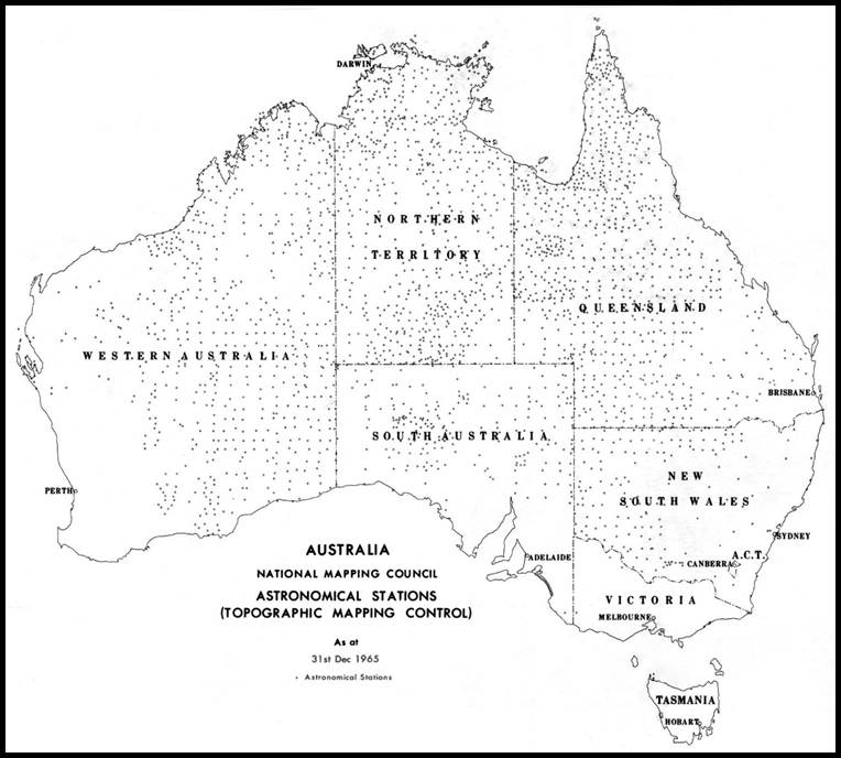
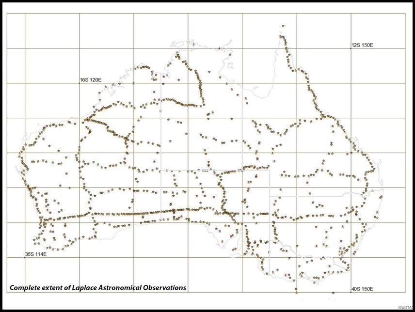
Where practicable, astrofixes were obtained in the vicinity of each intersection of the 4 mile map sheets, one in the vicinity of the centre of each 4 mile sheet, and one near each permanent feature such as homesteads, etc. During this program it was recorded that some 2 540 astrofixes were used for the R502 mapping program. The figure below shows the location of all astrofixes that were observed to 1965. In addition to the astrofix control established by the Royal Australian Survey Corps and National Mapping, each of the State mapping agencies of the time contributed as well as the following organisations :
Australian Gulf Oil Company Ltd
Delhi Australia Petroleum Pty Ltd
Department of the Interior
Hydrographic Office, Royal Australian Navy
Snowy Mountains Hydro Electric Authority
Country Roads Board, Victoria
Weapons Research Establishment, Department of Supply
Western Australian Petroleum Pty Ltd (WAPET).
In National Mapping many of the initial astrofix observers had served during the Second World War and were thus somewhat familiar with the stellar observation for Position Line. Position Lines were observed as cloudy skies, inexperienced observers, or the lack of star predictions did not impact the observation. The UK War Office methodology documented in the Textbook of Field Astronomy, 1958, was adopted by most. This method’s greatest drawback, however, was that the associated computations were laborious and time consuming. Nevertheless, it is understood that outside of National Mapping the majority of astrofixes were obtained by this method.
The basis of the observation for the traditional Position Line was that any two stars would give a position fix and any further stars observed would improve the fix. The result of all observations could be displayed graphically, and the effect of each observation could be assessed so that any doubtful observations became apparent and further observations made. More detail may be found at Annexure A.
At National Mapping an observation consisted of measuring four timed altitudes in quick succession to each of four stars lying approximately to the NE, SE, SW and NW. However, as longitudes were both more important and more difficult to obtain than latitudes, two additional stars lying to the east and west were included in every set of observations. Stars in opposite quadrants balanced each other in altitude and azimuth as well as possible, and were preferably observed consecutively. Stars lower than 30º in altitude were avoided if at all possible. Importantly bright stars only, brighter than magnitude 4.0, which would likely be listed in the Star Almanac, were observed. It was desirable to identify at least one or two of the brighter stars of an evening's program, particularly if an accurate azimuth was not available, ensuring the identity of the other observed stars could be found later. It was considered that an observation to one pair of latitude stars and two pairs of longitude stars would achieve a better result than an observation to any six stars.
At its inception in 1947, Natmap recruited George Robert Lindsay (Rim) Rimington (1908-1992) to the position of Chief Topographic Surveyor in the Photogrammetric Survey Sub-section of the then National Mapping Section. In that position Rim was directly responsible for the field activities conducted from the Melbourne office. Rim was thus part of the first field party which commenced the astrofix program in 1948. Dave Hocking’s 1985 account of Nat Map’s astrofix field work in the late 1940s and early 1950s was provided in his paper Star Tracking for Mapping. Rim bought with him what became known as Rimington’s Method of position fixing which enabled the Nat Map astrofix program, at least, to be expedited. Rim had developed his method while undertaking astrofix surveys for land administration, in the Northern Territory. In comparison to the traditional Position Line method Rimington’s method only took a couple of hours for the observations and a couple more to check its quality, meaning the field party could move on the next day.
Rimington’s Method depended on the assumed meridian being within a few minutes of the true meridian, and was designed so that each star was timed as it crossed the assumed meridian. During that time the star followed a course on which calculations could be made by the rules of simple proportion. (In Australia the meridian was set using the magnitude 5.42, close circum-polar star Sigma Octantis (Polaris Australis). Five pairs of north and south stars transiting the meridian, comprised a fix. The astrofix was accepted if three pairs of star observations were within 0.3 seconds of time (about 5 seconds of arc) for longitude and the latitude range for the north and south stars did not exceed five seconds of arc. The estimated reliability of an astrofix position by Rimington’s Method was about 100 metres. More detail may be found at Annexure B.
Ney Method
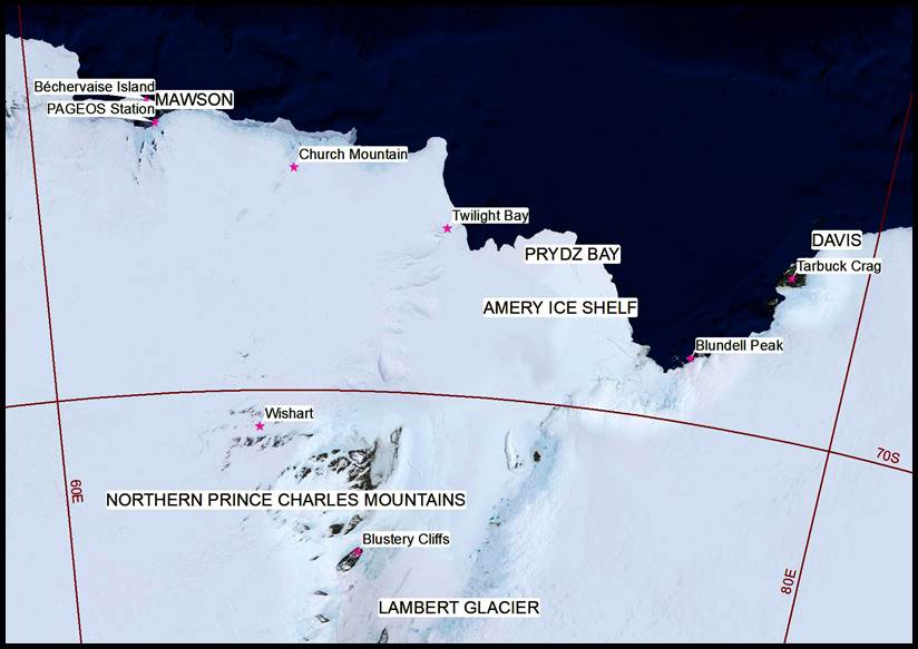
Named after Cecil Herman Ney (1889-1972) of the Geodetic Survey of Canada, his method recognised that in polar and subpolar areas, the rate of change of altitude per unit of time for any particular star was much less than in middle latitudes, affecting the accuracy of the subsequent stellar determinations. Furthermore, his observing procedure negated the problems of stellar altitudes being unable to be measured with the same degree of precision as horizontal angles and the difficulty of maintaining the theodolite telescope at a fixed vertical angle. His method had additional benefits for work in polar regions in that accurate instrument orientation was unnecessary as was a prepared observing program, and the observational work could be performed when only small parts of the night sky were free from cloud. While the Ney Method originated in the northern hemisphere it was equally applicable to the southern hemisphere, especially Antarctica, where it was used from time to time by Natmap surveyors. Below is a map and list of locations in Antarctica where observations by the Ney Method were known to have been acquired by Natmap surveyors.
|
IDENTIFIER |
NAME |
YEAR |
|
NMS54 |
Béchervaise Island |
1966 |
|
NMAS65 |
Church Mountain |
1967 |
|
NMAS54 |
Twilight Bay |
1968 |
|
NMAS73 |
Blustery Cliffs |
1969 |
|
NMAS74 |
Wishart |
1969 |
|
NMAS72 |
Blundell Peak |
1969 |
|
NMAS71 |
Tarbuck Crag |
1969 |
|
ISTS051 |
PAGEOS Station |
1971 |
The basis of the Ney Method was that from timed azimuth observations on at least three stars, and operationally as many as could be managed in an observing program, latitude, longitude, and azimuth could be derived simultaneously. With three unknowns, latitude, longitude, and azimuth, the solution required the minimum of three observations but with more stars and using least squares the derived values were improved.
Complete details, including an observation and its numerical reduction, was provided by Ney in his 1954 paper Geographical Positions from Stellar Azimuths (Ney, 1954).
Recollections on the use of Daylight Stars and the Ney Method by Max Corry, former National Mapping Antarctic Surveyor, may be read at Annexure G.
The Laplace Observation
Commencing in 1950 and continuing until around the early 1980s stellar observations were acquired at specific previously established geodetic stations to determine their astronomic latitude, longitude and azimuth. Differences between a station’s geodetic and astronomic coordinates enabled information to be derived about the mathematical spheroid and the real world surface (geoid) at that station. The stations for which both astronomic and geodetic (astro-geodetic) coordinates were known were called Laplace stations. Pierre-Simon, marquis de Laplace (1749–1827) developed the relationship as the amount of local deflection could not be measured directly and was thus deduced by a comparison of the astronomic position obtained by stellar observation, with the geodetic position computed with reference to the spheroid which best represented the form of the whole earth or a particular part of it. More on Laplace’s equations is at Annexure C.
To obtain astronomical latitude and longitude to the greatest accuracy possible, a star was observed near the meridian where an error in longitude had the least effect on a latitude observation whereas an observation for longitude was taken with a star near the prime vertical, where an error in latitude had least effect. The specific stellar observations to achieve this was an almucantar (when two objects are on the same almucantar, they have the same altitude) observation for longitude and latitude by circum-meridian altitudes. Azimuth was derived from observations on the magnitude 5.42, close circum-polar star Sigma Octantis.
Almucantar observation for Longitude (see also Annexure D)
The theodolite needed to be fitted with a graticule having 5 horizontal intersections on the vertical wire, each 5 minutes of arc apart (i.e. two above and two below the central horizontal cross-hair). Time was recorded using either a high quality split hand type stopwatch with a large dial, clear figures and graduated to 1/10 of a second so that 1/100 of a second could be estimated, or timing equipment allowing the observer to record the time of observation on a paper chart along with regular timing marks.
Any east star could be paired with any west star, providing they were observed within twenty minutes of time. The aim was for 16 pairs of stars, 8 on each of 2 nights; the minimum was 12 pairs of stars with not less than 6 pairs on each of 2 nights. Available stars were predicted in advance for the location with altitudes of around 30º.
The essence of the observation was timing a star across the series of 5 hairs and at each instant reading the alidade bubble. No angles needed to be read and the only theodolite movement was with the ex-meridian footscrew to vary the bubble and the horizontal slow motion screw to keep the star close to the vertical wire as it cut the five horizontal wires.
Latitude by Circum-Meridian Altitudes (see also Annexure E)
Pairs of stars were selected in advance of the observation. They were paired north and south within 4° of altitude and 20 minutes of time, tedious until computers was trying to find a partner among the many north stars for each of the rarer south stars.
Observations on a single night were acceptable but 8 pairs of stars on each of two nights was the aim, 12 pairs of stars being the minimum. Six shots were required per star, the maximum time allowed in which to complete these was six minutes, i.e. three minutes each side of upper transit. Overall it was considered better to obtain a few shots to many stars, than many shots to a few stars. The theodolite observations were all acquired on the same theodolite face and balanced with similar observations on another star of equivalent altitude which was 180° from the star initially observed.
Azimuth from a close Circumpolar Star (see also Annexure F)
With a declination of approximately 89° 04'S and its fastest movement in azimuth (at upper or lower transit) being only some 17 seconds of arc in 1 minute of time, observing the close circum-polar star Sigma Octantis was not difficult and time was only needed within a half second accuracy. Azimuth from Sigma Octantis was thus a routine observation in National Mapping.
For best results at least six sets, three on each of two nights, was required but a single night’s observation of one set of six zeroes, was considered sufficient for checking azimuth.
Frequency and Significance of the Laplace Observations in Australia
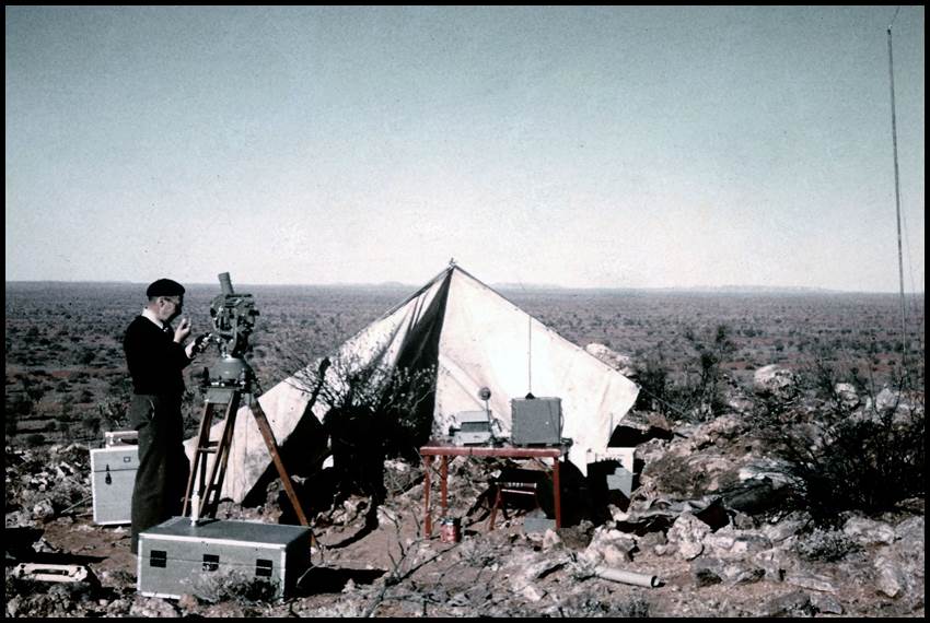
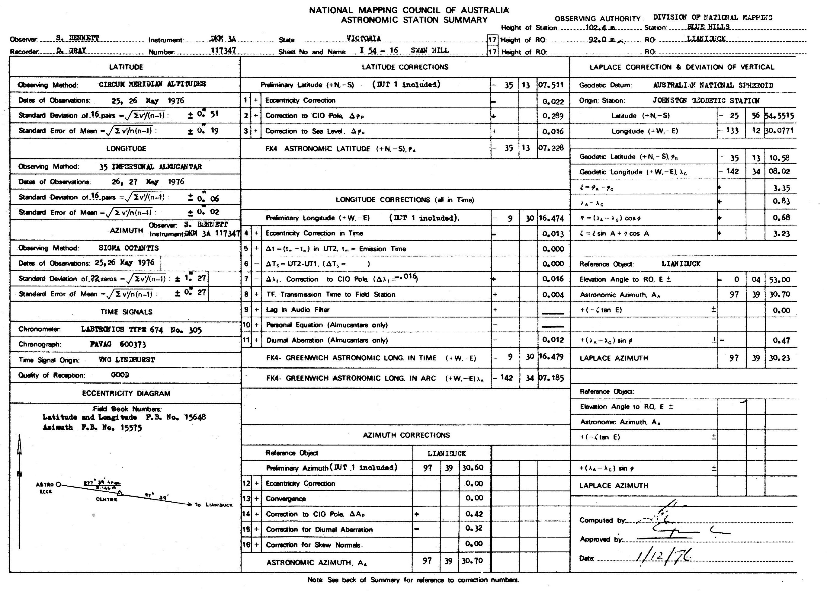
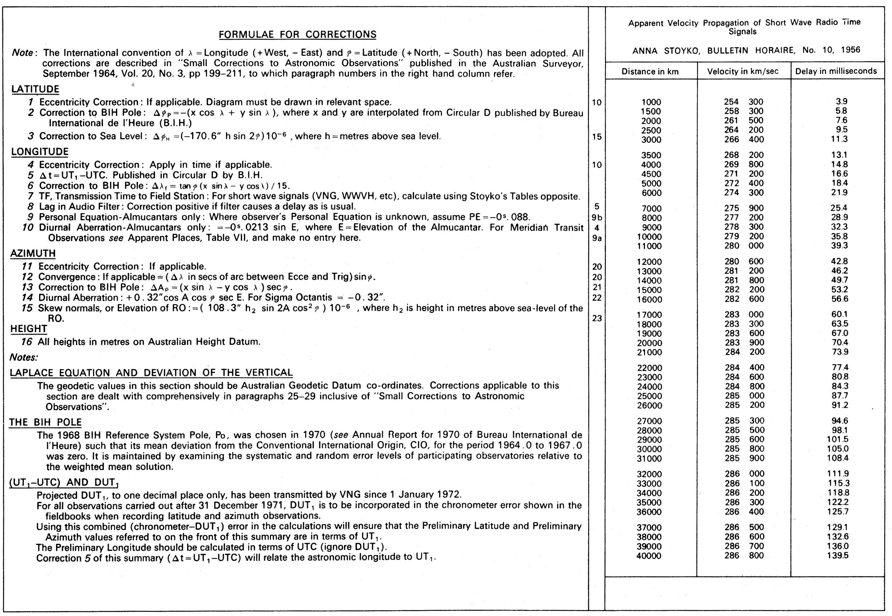
As described above a Laplace observation consisted of three discrete observations carried out at existing geodetic survey stations for the purpose of determining astronomic latitude, longitude and azimuth. The photograph below shows a Wild T4 theodolite and requisite timing equipment during a Laplace observation by Natmap’s Dr Peter Bardulis. For azimuth control, as defined by equations (2) & (3) in Annexure C, only the longitude and azimuth observations were required. If the deflectionof the plumb line was required to be known in both directions, however, as for geoidal studies, then the latitude observation was also required.
The then National Mapping Director Bruce Lambert outlined in his 1964 paper The Role of Laplace Observations in Geodetic Survey the use of Laplace observations in the Australian context. As well as correcting for any azimuth errors in the geodetic survey, the astro-geodetic differences at Laplace observation stations could be analysed to determine appropriate parameters for a mathematical reference surface or spheroid and the latitude and longitude coordinates of its origin.
This was at a time when the reference surface or spheroid used for the geodetic calculations for the Australian Geodetic Survey was taken from those already published, mainly for the northern hemisphere. A specific spheroid for Australia had yet to be defined but would evolve from the astro-geodetic work already in progress.
Bessel‘s 1841 and Clarke’s 1858 spheroids were among those initially used in Australia. Their use meant that Tables of Geodetic Constants existed, which saved a significant amount of computational work in the calculation of the geographical coordinates from the geodetic survey work. The Bessel spheroid was first derived in 1837 by Friedrich Wilhelm Bessel (1784-1846), and was based on meridian arcs totalling some 50 degrees and having 38 precise measurements of astro-geodetic latitude and longitude. In its day Bessel’s determination was then considered the best and with the most modern data for mathematically describing the Earth's figure. Bessel’s 1841 values were an equatorial radius a of 6 377 397 metres and flattening f of 1: 299.2. Alexander Ross Clarke (1828-1914) was recognised for his calculation of the Principal Triangulation of Britain (1854-1858). Clarke’s results came from using nine of the same ten meridian arcs as used by Bessel, some with improved data. Clarke’s 1858 values were an equatorial radius a of 6 378 293 metres and flattening f of 1: 294.3. (A meridian arc is the measurement of the distance between two points with the same longitude. Parallel arcs could also be measured between two points with the same latitude but it was the meridian arc that became the most useful in deriving a mathematical figure of the Earth.) Initial calculations in Australia in National Mapping used Clarke’s 1858 values with the coordinates of the Sydney Observatory (33º 51’ 41.10” S 151º 12’ 17.85” E) accepted as the origin.
Lambert explained that once a significant number of astro-geodetic stations existed their coordinate differences could be analysed to determine more appropriate parameters for the mathematical reference spheroid. The analysis, best done using a least squares process to eliminate systematic effects introduced by the use of a wrong reference spheroid, wrong starting latitude, longitude and azimuth, and also for the purpose of reducing the squares of the residual deflections to a minimum. The process would be repeated as more observations were acquired, until stability was achieved.
Further, because gravity was variable, depending upon things such as variable Earth mass, the geoid was an irregular surface. Thus a 10 to 15 mile grid pattern of astro-geodetic observations was seen to be needed to establish a reasonably accurate Australian geoid contour pattern. (The Geoid was an imaginary surface which coincided closely with mean sea level over the ocean and its extension under the continents.) In practical terms the difference between GPS and Australian AHD height was the geoidal height. As such a network of astro-geodetic values was not likely to be available for some considerable time, as an interim measure, selected geoid profiles would first be observed. From these, elevations could be deduced and analysed to provide initial values.
At the time of Lambert’s writing, Laplace observations, acquired at every six geodetic stations on average, had already been used for the purpose of arriving at provisional origin coordinates and a reasonably fitting spheroid. It, however, would be many years before geoid sections, let alone a complete geoid contour map, would be available as the National Mapping Council had specified that the final spacing between Laplace observations should be 4 to 6 stations. The specifications and recorded operational practices of the time, reflected Lambert’s remarks.
The earliest National Mapping Council of Australia Standard Specifications for Horizontal and Vertical Control, of 1953 (National Mapping Office, NMO/53/11.2), stated that a Laplace station shall be established at a triangulation station situated approximately at the mid point of each chain of triangulation connecting pairs of base lines (noting that at that time triangulation was the established geodetic survey methodology). Nevertheless, traversing was not overlooked as the specifications also stated that Laplace stations shall be established at approximately 100 mile intervals along traverses, or at such closer intervals as are considered necessary to eliminate errors caused by gravity anomalies.
The National Mapping Council of Australia later published Standard Specifications and Recommended Practices for Horizontal and Vertical Control Surveys (Special Publication 1, 1966, revised 1976 and 1981). Therein it was stated that the determinations of azimuth as well as longitude should be distributed in at least three different nights. In traverse and triangulation nets as well as trilateration nets with angle measurements along traverses joining the Laplace stations, a simpler rule might be sufficient, giving the permissible number of azimuth transporting angles between two Laplace stations as a function of the accuracy of horizontal angle measurements and astronomic measurements. The highest number of azimuth transporting angles between Laplace stations might be put as 8-10 in triangulation and 6 or less in traverse work (more simply every 8-10 stations in a triangulation or at least every 6th station on a traverse).
Operationally there is information that a Laplace observation was undertaken every six stations during the 1959 work of Frank Johnston (McLean, 2017). By 1963 Laplace work by Klaus Leppert was undertaken at least every fourth line. In both these examples all three discrete observations were undertaken.
As far as it is known, specific programs of Laplace observations like the two just mentioned included the full set of astronomical observations giving astronomical latitude, longitude and azimuth. During the completion of various long traverse loops, however, Laplace observations likely consisted of just astronomical longitude and azimuth to monitor the geodetic azimuth of the work.
The Australian Geodetic Datum, 1966 (AGD66) and the Australian National Spheroid (ANS)
Laplace observations were integral to the development of a spheroid that best fitted Australia. From a comparison of the astro-geodetic coordinates at 54 Laplace stations in the vicinity of the 32º parallel between Sydney and Perth, the Maurice origin emerged. Trigonometrical station Maurice was on Maurice Hill some 16 kilometres south west of Orroroo, South Australia. The necessary geodetic computations were performed using the NASA (United States, National Aeronautical and Space Administration) spheroid. As a result of these computations, new central origin and spheroidal parameter values were determined and from April 1963 to April 1965 computations were made on the “165” spheroid with the “165” central origin. The “165” central origin was based on the astro-geodetic comparison of the coordinates at 155 Laplace stations spread over the whole of Australia with the exception of Cape York and Tasmania. In 1965 the International Astronomical Union adopted the parameters of a spheroid for astronomical use. The National Mapping Council was satisfied that these parameters were also an appropriate fit for Australia and adopted these values for the Australian National Spheroid (ANS).
In May 1965, a complete recomputation of the geodetic survey of Australia commenced, emanating from trigonometrical station Grundy, whose coordinates on both the “165” spheroid and the Australian National Spheroid were 25° 54' 11.078"S and 134° 32' 46.457"E. Trigonometrical station Grundy was on Mount Grundy about 35 kilometres south of Finke in the Northern Territory and 135 kilometres almost due east of the later determined Johnston Geodetic Station. It is now interesting to note that Mount Grundy is less than 50 kilometres south of the Lambert Gravitational Centre that was determined in 1988 and named after Bruce Philip Lambert, the longest serving Director of National Mapping.
By December 1965, further Laplace observations had also been undertaken to then include Cape York and Tasmania, bringing the total number of Australian Laplace stations to 533. Of these Laplace stations, 275 stations were judiciously selected and an astro-geodetic comparison of their coordinates revealed that :…random undulations in the geoid make it impossible to locate a centre for the spheroid with a standard error of less than 0.5 seconds [of arc], about 15 metres, even with a very large number of stations. This finding saw the central origin calculated using these 275 Laplace stations being adopted as the best available at the time. Thus, as resolved by the National Mapping Council the coordinates of this central origin would determine an area in which the Johnston Geodetic Station, or Johnston Origin, could be located. Its centrality later gave this point notoriety as the first calculated centre of Australia!
The major parameters of the various abovementioned spheroids, plus WGS72 for comparison purposes, were :
|
Spheroid name |
Semi-major (equatorial) axis (a) |
Flattening 1/f |
|
Bessel 1841 |
6 377 397 metres |
299.16 |
|
Clarke 1858 |
6 378 293 metres |
294.26 |
|
NASA |
6 378 148 metres |
298.3 |
|
“165” |
6 378 165 metres |
298.3 |
|
ANS |
6 378 160 metres |
298.25 |
|
WGS72 |
6 378 135 metres |
298.26 |
The 1966 national adjustment of the Australian Geodetic Survey comprised some 2 506 stations, 53 000 kilometres of Tellurometer traverse, the geodetic triangulation nets, and 533 Laplace stations. The raw survey data was converted into a continental wide series of very accurately related coordinates in latitude and longitude. This adjustment used the ANS with its central origin at the Johnston Geodetic Station, in photograph below, having the three dimensional coordinates of :
Latitude: 25° 56' 54.5515" S
Longitude: 133° 12' 30.0771" E
Elevation: 571.2 metres above the Spheroid
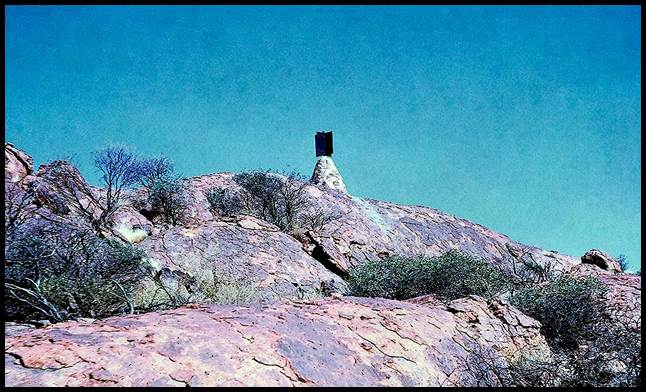
The Johnston Origin, together with the adopted spheroid then provided the basis for the Australian Geodetic Datum (AGD66), and this datum was adopted by the National Mapping Council on 21 April 1966, and proclaimed in the Commonwealth Gazette No.84 on 6 October 1966.
The Australian Geoid
As mentioned by Lambert above, having established a continental spheroid the next stage was to establish the Australian Geoid. As an interim measure, selected geoidal profiles would first be observed to provide initial values. As further observations were acquired the geoid would be improved.
The term geoid is used to describe the equipotential surface of the Earth; the surface of the Earth's gravity field which best corresponds with mean sea level. In the context of a figure of the Earth, the spheroid is a mathematical shape that best fits the geoid overall. Owing to variations in the composition and density of the Earth’s crust, differences in mass will cause the geoid to dip below or rise above the surface of the spheroid. In Australia where heights are related to the Australian Height Datum (AHD) the AHD is about 0.5 metres above the geoid in northern Australia and roughly 0.5 metres below the geoid in southern Australia.
A geoid was first established in Australia, from Laplace observations and an astro-geodetic analysis, for the Woomera region in South Australia. A continental astro-geodetic geoid for Australia was first produced by the United States Army Map Service in late 1966 and referred to the Australian Geodetic Datum. This 1966 geoid was based on Laplace observations recorded at approximately 600 geodetic stations and was known as the 1967 astro-geodetic solution. A further solution was derived by Nat Map in 1971. The 1971 solution used the astro-geodetic observations from 1 133 Laplace stations. The field work component of this program together with earlier astronomical observation activities, was largely complete by 31 December 1970 and included astronomical reobservations at 110 stations during 1966-1970.
The first stage of the 1971 work was the computation of sections of primary geoidal profiles along traverses where the astronomical station spacing was generally less than 35 kilometres. These sections formed large loops which were broken up by geoidal profiles along traverses where the astronomical stations spacing was often in excess of 50 kilometres. A weighted least squares adjustment provided values of N for 1 133 astro-geodetic stations.
Values of N and the deflections of the vertical were gravimetrically computed at 51 geodetic stations and at 1 679 points on a half degree grid inside the loops formed by the geoidal profiles. The gravimetrically computed values were adjusted, loop by loop, into the system defined by the adjusted values of N at the astro-geodetic stations on the loop perimeter. A total of about 3 000 values were available for the automatic contouring of maps of the deflections of the vertical and N.
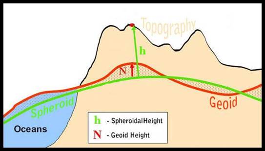
In the diagram below, the height H of the point in the topography above the geoid was considered to be close to the AHD value within ±0.5 metres and h was the height of the point above the spheroid, which would be obtained using GPS. The Geoid-Spheroid separation or N value was thus N = h -H.
The offset between the AHD and the geoid in Australia was caused predominantly by the difference in ocean temperature between northern and southern Australia. In establishing the AHD, the mean sea level at 32 tide gauges from all around the Australian coastline were assigned a value of 0.000 metres AHD. The warmer/less dense water off the coast of northern Australia was approximately one metre higher than the cooler/denser water off the coast of southern Australia, causing the ±0.5 metre difference.
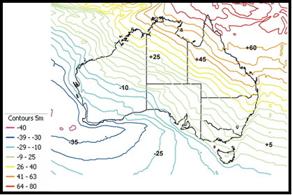
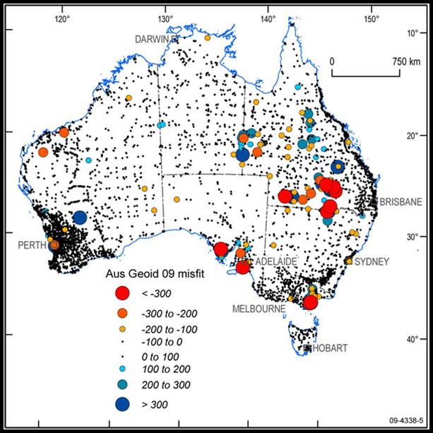
The advent of height from GPS then saw the need for such heights to be related to the Australian Height Datum. GPS heights were spheroidal heights and found to differ from geoid/AHD heights by between -30 and +70 metres across Australia. This was known as the geoid-spheroid separation, or N value. To convert ellipsoidal heights to geoid/AHD heights, a geoid model can be used. It is important to be clear that GPS heights are not AHD heights and must be used with caution. The plot below is a visual geoid model where the contours show the Geoid-Spheroid separation (N value) where a positive value means the spheroid is above the geoid. If a GPS/spheroid height was read as 75 metres along the +5 metre (green) contour then the AHD/geoid height would be 70 metres (75-5 metres).
To improve the accuracy in converting GPS height to AHD, a geometric component was developed from GPS and AHD data which described the approximate one metre offset trend and combined the gravimetric and geometric components into a single national grid with two kilometre resolution. This geoid was now not truly an equipotential surface but the practical result obtained over-rode a theoretical concept.
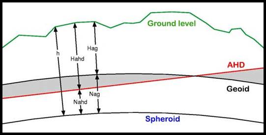
In the diagram below four surfaces are diagrammatically depicted. Ground level is the topographic surface and the mathematical surface used for geodetic geographic calculation is the Spheroid. In Australia there is the surface to which all heights are related, the Australian Height Datum (AHD) and finally the Geoid. The offset (O) between the AHD and the gravimetric geoid, which is positive when the AHD is above the gravimetric geoid, was derived at over 5 000 points across Australia; O = h – Nag – Hahd where h is the spheroidal height (from GPS observations), Nag is the gravimetric geoid - ellipsoid separation (from the gravimetric geoid), and Hahd is the AHD height.
Around 2001, GPS/spheroidal heights could be converted to an AHD height within ±0.364 metres across 65 per cent of Australia. By 2009 the conversion accuracy had been reduced to less than ±0.050 metres. It should be noted however, that in some less populated areas large misfits still exist in some areas as depicted in the diagram below (units in millimetres).
The AUSGeoid2020 model now provides the offset between the GDA2020 ellipsoid and the Australian Height Datum (AHD). This tool can transform between ellipsoidal (GPS) and AHD heights and supplies uncertainty estimates. The conversions are valid (on-shore only) for latitude and longitude coordinates between 8ºS to 61ºS and 93ºE to 174ºE. The input coordinate format is decimal degrees.
The results are tabled as :
|
Criteria (repeat of input values) |
||
|
Latitude |
Longitude |
Ellipsoidal Height |
|
Results |
||
|
AHD Height |
AHD Uncertainty |
Ellipsoid to AUSGeoid2020 Separation |
|
|
|
|
|
Deflection of the Meridian |
Deflection of the Vertical
|
|
providing not only the AHD height for the location but an indication of its accuracy. Also is information for the location that once only came from a Laplace observation at that spot.
Closing remark
The stellar observation programs of National Mapping led to the first national map coverage being achieved as quickly as possible and surveys in Australia and Antarctica being of a consistently high order. The much longer Laplace programs led to the Australian Spheroid being established, followed by iterative improvements in the knowledge of the Australian Geoid and its relationship to the Australian Height Datum and spheroidal/ellipsoidal datums.
Acknowledgement
Information from the websites of Geoscience Australia (GA) and the Intergovernmental Committee on Surveying and Mapping (ICSM), is gratefully acknowledged.
Paul Wise, April 2022.
Some notes on the Observation to Daylight Stars
National Mapping observed daylight stars for position fixing in Antarctica and azimuth in Australia. In his article Groundmarking for Aerodist – 1969, August Jenny described his recollections of azimuth determination by observing daylight stars at elongation. Daylight stars in the southern hemisphere used by Natmap are known to have been :
|
Catalogue Number |
Name |
Apparent magnitude |
|
179 |
α Carinae (Canopus) |
0.6 |
|
32 |
α Eridani (Achernar) |
0.5 |
|
340 |
1.3 |
|
|
364 |
β Centauri |
0.6 |
|
379 |
α Centauri |
0.1 |
|
328 |
α Crucis |
0.8 |
As daylight stars could only be seen in the theodolite telescope the approximate position of the star had to be computed beforehand to enable it to be found for subsequent observation. Natmap, recollected Jenny, had provided very convenient nomograms to assist with the prior determination of a star’s azimuth angle, zenith distance and hour angle at elongation, graphically. Bennett (1974), Camm (1957) and Thornton-Smith (1955) produced papers which dealt with the prediction of daylight stars. Interestingly both Bennett and Thornton-Smith, did not include β Crucis in their works possibly as it was considered too bright for some precise observations.
Position Line Observation
The basis of the observation for the traditional Position Line was that any two stars would give a fix and any further stars observed would improve the fix. All observations could be displayed graphically, and the effect of each observation could be assessed so that any doubtful observations became apparent and further observations made.
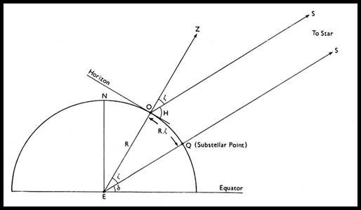
Theoretically, the observer at O on the surface of the earth measured the altitude H of a star S, as shown in the diagram above, with the vertical plane through O and S. Assuming a spherical earth this included the centre E. If Z was the zenith of O, the zenith distance ZOS of the star equalled 90° - H. Since S was very distant, the directions of the star at O and E were considered parallel, hence the angle ZES also equalled 90° - H.
If ES met the surface of the earth at Q, Q was the point directly beneath the star and the star lay at the zenith of Q. Q was known as the sub-stellar point.
The angle OEQ = angle ZOS = 90° - H
The observation thus defined the distance (in arc) of O from a point Q. The locus of O was therefore a circle centre Q, and this was known to the observer as a position circle; its centre was the sub-stellar point, its radius in arc 90° - H, and it was a small circle of the sphere, on which it is shown in the figure below.
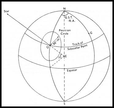
Owing to the rotation of the earth, the same point on its surface did not remain beneath a star; the sub-stellar point for that star moved round the earth with the star, but its latitude remained constant, and equal to the declination of the star. For EQ in the above figure made the same angle δ with the equatorial plane as did ES. The sub-stellar point therefore moved along a parallel of latitude.
The longitude of Q may be instantaneously defined, for Q must lie in the same meridian plane as the star; the longitude QNG of Q was then equal to the Greenwich Hour Angle (GHA) of the star, which could be derived provided that the time of observation was known :
Then West Longitude of Q = GHA Star = Greenwich Sidereal Time (GST) - Star's Right Ascension (RA)
The circle of radius 90° - H and centre Q was all that could be deduced from a single observation of a star. At any point on the circle, however, the direction of the adjacent part of its circumference could be ascertained, since it must be perpendicular to its radius. Hence the direction of the position line at any point thereon must be perpendicular to the direction of the sub-stellar point, which was also that of the star. As an approximate position of the observation was known, only the location of the position line in the immediate neighbourhood was of interest. The position line could thus be considered a straight line perpendicular to the star observed.
If another star was observed its position circle intersected that of the first star at two places but was obvious which intersection is the one indicating the observer’s position. The observation of further stars added further position circles which improved the solution for determining the most likely coordinates for the observer’s position.
Rimington’s Method
Rimington’s Method depended on the assumed meridian being within a few minutes of the true meridian, and was designed so that each star was timed as it crossed the assumed meridian. During that time the star followed a course on which calculations could be made by the rules of simple proportion. (In Australia the meridian was set using the magnitude 5.42, close circum-polar star Sigma Octantis (Polaris Australis). Five pairs of north and south stars transiting the meridian, comprised a fix. The astrofix was accepted if three pairs of star observations were within 0.3 seconds of time for longitude and the latitude range for the north and for the south stars did not exceed five seconds of arc. The estimated reliability of an astrofix position by Rimington’s Method was about 100 metres.
The theory is that for two stars which transit in the north & south respectively let :
z1 and z11 = zenith distances of N & S stars at transit
δ1 and δ11 =declinations of N & S stars
dt1 and dt11 = corrections to N & S stars due to error in assumed meridian
dA = azimuth correction due to error of assumed meridian.
When a star is very close to the meridian, the following relationship holds good as dA is small :
dt1 = dA sin z1 sec δ1 (1)
dt11 = dA sin z11 sec δ11 (2)
dividing (1) by (2) :
dt1/dt11 = sin z1 sec δ1 / sin z11 sec δ11
Obtaining T (in seconds of time) = dt1 + dt11, that is the amount of time obtained by subtracting the difference of RAs of N & S stars of a pair from the difference of their Chronometer times of transits, the Chronometer times corrected to Sidereal, then
dt1 = T sin z1 sec δ1 / [sin z1 sec δ1 + sin z11 sec δ11]
dt11 = T sin z11 sec δ11 / [sin z1 sec δ1 + sin z11 sec δ11]
By adding (1) and (2), and transposing :
dA (Seconds of Arc) = 15T / [sin z1 sec δ1 + sin z11 sec δ11]
Thus when T is known, the values of dt1, dt11 and dA are obtained by the rule of simple proportion.
Corrections for the difference between assumed and true meridian are made to the times of transit of the stars to give Local Sidereal Time of transit which minus Greenwich Sidereal Time of transit equals longitude expressed in time.
By recording the times the star crossed the horizontal stadia wires, early stadia face right and late stadia face left with the mean giving time of transit of the assumed meridian and reading the zenith distance, ZD, on face left, a simple calculation of ZD plus correction for refraction and the star's declination gave latitude.
More detail with worked example are in Training Notes for National Mapping Field Survey Staff compiled by Reg Ford.
Laplace Equations
Pierre-Simon, marquis de Laplace (1749–1827) developed the relationship as astronomical determinations of position included the effect of local deviations caused by the irregular distribution of mass in the earth's crust. The amount of local deflection could not be measured directly and was usually deduced by a comparison of the astronomic position obtained by stellar observation, with the geodetic position computed with reference to the spheroid which best represented the form of the whole earth or a particular part of it.
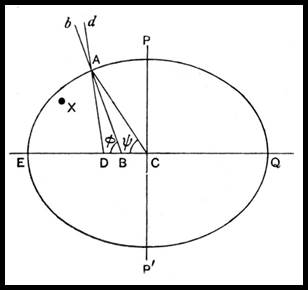
The difference between the geodetic and the astronomic latitude is illustrated in the above figure. The curve EPQP’ represented a section through a meridian on the earth's surface, PP' being the polar axis and EQ the equatorial axis. Since the earth was taken as an oblate spheroid in shape, this curve was an ellipse. At any point A the line bAB was drawn normal to the curve at A and A was joined to C, the centre of the ellipse. Then the angle ACE was the geocentric latitude ψ and the angle ABE was the geodetic latitude φ.
If an abnormally heavy mass was now concentrated at the point X, a plumbob suspended at A was then drawn by gravitational attraction towards X, so that the plumb line was no longer along the normal bAB but along some other line say dAD. As all astronomic observations for latitude ultimately depend on the indications of a spirit level, and, as a level plane was indicated when the bubble was at the centre of its run, its tangent plane was thus perpendicular to the plumb line. The latitude measured by the instrument was the angle ADE and not the geodetic latitude ABE. The measured latitude ADE was called the astronomic latitude, and the difference between this and the geodetic latitude, the angle BAD in the figure, was called the deviation of the vertical, or of the plumb line, in latitude. If the mass X was to one side of the meridian plane, and not exactly on it, there would be a similar deviation in the local time, so that the astronomic longitude LA did not coincide with the geodetic longitude LG. When the point of observation was not on the equator this difference between astronomic and geodetic longitudes led to a difference between the astronomic and geodetic azimuth, since the effect was to slightly tilt the plane in which the horizontal angles were measured.
Essentially, astronomic observations of directions to stars are gravity based and yield astronomic positions. Survey (azimuth and distance from a known point to an unknown point) derived positions are spheroidal based and provide geodetic positions. Further, the spheroidal surface is not necessarily parallel with the level surface of the terrain or geoid. The angular amount by which the two surfaces are not parallel is given by the deflection of the vertical and is expressed in terms of a north/south or in meridian component and an east/west or in prime vertical component.
Laplace related the two systems such that :
the deflection in meridian (ξ or east/west direction)
= Astronomic latitude - Geodetic latitude (1)
the deflection in prime vertical (η or north/south direction)
= (Astronomic longitude - Geodetic longitude) cos (Geodetic latitude) (2)
OR
= (Astronomic azimuth - Geodetic azimuth) cot (Geodetic latitude) (3)
His equations (2) and (3) showed that deflection in prime vertical (η) could be deduced from the difference of either the astronomic and geodetic longitudes or the astronomic and geodetic azimuths. As the two values for η must be the same then combining equations (2) and (3) gave :
Geodetic azimuth - Astronomic azimuth =
[(Astronomic longitude - Geodetic longitude) sin (Geodetic latitude)] (4)
Equation (4) is most important as it enabled the geodetic azimuth at any Laplace station to be determined from a combination of astronomic azimuth and longitude observations. Laplace stations therefore permitted an independent check to be made on a survey’s derived geodetic azimuth.
Further if the line joining two stations has an azimuth A, then the component of deviation in azimuth A (χ) in seconds of arc
= - (the deflection in meridian (ξ) * cos azimuth (A)) + (Geodetic longitude * sin azimuth (A))
Thus if two geodetic stations (Station a and Station b) at which the Laplace observations have also been undertaken are distance L apart and N is the height of the geoid above the spheroid, the difference in geoidal height (ΔN) between Stations a and b is (Nb – Na) where :
ΔN = Nb – Na = + ½ (Χ"b + Χ"a) * L * sin 1" (ΔN in the same units as L) (5)
Although Formula (5) is an approximation it has been operationally shown that unless the geoid is unduly disturbed, satisfactory values for ΔN can be economically obtained if L is about 15 miles (or about 25 kilometres).
Annex B of the 1981 National Mapping Council of Australia, Standard Specifications and Recommended Practices for Horizontal and Vertical Control Surveys, contained a sample Astronomic Station Summary showing a sample Laplace observation methodology and reduction.
Almucantar Observation for Longitude
The theodolite needed to be fitted with a graticule having 5 horizontal intersections on the vertical wire, each 5 minutes of arc apart (i.e. two above and two below the central horizontal cross-hair). Time was recorded using either a high quality split hand type stopwatch with a large dial, clear figures and graduated to 1/10 second so that 1/100 second could be estimated, or timing equipment allowing the observer to record the time of observation on a paper chart along with regular timing marks.
Any east star could be paired with any west star, providing they were observed within twenty minutes of time. The aim was for 16 pairs of stars, 8 on each of 2 nights; the minimum was 12 pairs of stars with not less than 6 pairs on each of 2 nights. Available stars were predicted in advance for the location with altitudes of around 30º, theodolite dependent.
The theodolite was set so that two footscrews were along the line of the meridian. This arrangement allowed the alidade bubble to be altered slightly after each timing of a star, by moving the ex-meridian footscrew. The star altitude selected for the prediction plus refraction was then set on the vertical circle, which then remained clamped throughout the observations.
The essence of the observation was timing a star across the series the 5 hairs, at each instant reading the alidade bubble. No angles needed to be read and the only movement was with the ex-meridian footscrew to vary the bubble and the horizontal slow motion screw to keep the star close to the vertical wire as it cut the five horizontal wires.
For the computation the set altitude plus refraction angle was used along with the mean of the five alidade bubble readings converted to time.
In the spherical triangle where Z was the Zenith, P was the south celestial Pole and S was the star crossing the Almucantar circle, longitude was calculated by solving for the Hour Angle (HA) with the following known :
z = ZS = 90º - Altitude (from the Almucantar Circle setting used set for the observation);
c = ZP = 90º - Latitude (from the Latitude Observation or known latitude)
p = 90º - Declination of observed star.
The Tan formula was most suitable because of its more sensitive value giving :
Tan(HA/2) = √{ (sin(s-c)*sin(s-p)) / (sin s * sin(s-z)) }
where (HA/2) = half the Hour Angle.
More detail with worked example are in Training Notes for National Mapping Field Survey Staff compiled by Reg Ford.
Latitude by Circum-Meridian Altitudes
Pairs of stars were selected in advance of the observation. They were paired north and south within 4° of altitude and 20 minutes of time.
Observations on a single night were acceptable but 8 pairs of stars on each of two nights was the aim, 12 pairs of stars being the minimum. Six shots were required per star, the maximum time allowed in which to complete these was six minutes, i.e. three minutes each side of upper transit. Overall it was considered better to obtain a few shots to many stars, than many shots to few stars. The theodolite observations were all acquired on the same theodolite face and balanced with similar observations on another star of equivalent altitude which was 180° from the star initially observed.
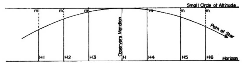
The basis of the observation was that, as shown above, when a star was close to transit, the small circle of altitude and the horizon could be considered parallel lines, as also could the star altitudes H and H1 to H6. The calculation involved finding the correction m for each observation so that when m was added to the observed altitude, the result was as though the actual observations were all taken at the time of transit. Knowing longitude, the time of transit of the star could be found and the time of each observation was recorded. Using the small time difference between times of observation and transit, (i.e., Hour Angle) m could be found in Star Catalogues and was derived from :
Correction (seconds of arc) = 2*Sin2(½HA) / Sin 1" where ½HA is in seconds of arc.
As m is affected by the latitude and also the declination and altitude of the star, m from the table must be multiplied by a factor k obtained from :
Cos Latitude x Cos Declination x Secant Altitude
The calculation was easy but must be methodically laid out as a separate m for each of the six observations must be read from the Table and then multiplied by k before applying the correction to each of the observations.
More detail with worked example are in Training Notes for National Mapping Field Survey Staff compiled by Reg Ford.
Azimuth from Observations on a Close Circumpolar Star
With a declination of approximately 89° 04'S and its fastest movement in azimuth (at upper or lower transit) being only some 17 seconds of arc in 1 minute of time, observing the close circum-polar star Sigma Octantis was not difficult and time was only needed within a half second accuracy. Azimuth from Sigma Octantis was thus a routine observation in National Mapping.
For best results at least six sets, three on each of two nights, was required but a single night’s observation of one set of six zeroes, was considered sufficient for checking azimuth.
Reduction of the observations consisted of finding how far the star was from 180º (due south) at time of observation i.e. the azimuth of Sigma Octantis was 180º ± A where :
A" = ((206264.8 *sine t) / (a-(b * cos t))) and a = sin and b = (sin dec * cos / cos dec) and
A" = Azimuth Angle in seconds or arc
p" = Polar Distance in seconds of arc
t = Hour Angle
= Latitude of station.
More detail with worked example are in Training Notes for National Mapping Field Survey Staff compiled by Reg Ford.
p class=MsoNormal>
The Use of Daylight Stars and the Ney Method
Recollections by Max Corry, former National Mapping Antarctic Surveyor
From email of 6 May 2022
Daylight Stars
…it seems to have been introduced in Antarctica by Australia in the mid to late 1950s and the US adopted this a couple of years later, after learning about the Australian use of daylight stars.
General survey instructions included in the 1965 surveyor’s instructions had the following : In high southern latitudes there is not a wide selection of stars of suitable magnitude; those commonly used are Alpha and Beta Centauri, Alpha Crucis, Canopus, Sirius, Fomalhaut, Achernar, Spica, Antares and Rigel.
The Ney Method
As mentioned, Ney’s Method originated in Canada with the U.S. first using it in Antarctica [as follows] :
Since the 1960-1961 season, the primary means of astronomic position determination has been by daylight stellar observations, using a method first described by C. H. Ney of the Geodetic Survey of Canada. This method is based on the movement of stars in azimuth, and accordingly vertical refraction is not a factor in the results. Latitude, longitude, and azimuth may be determined simultaneously by obtaining observations on a minimum of three stars. In practice, however, at least eight stars are usually observed and, in some cases, such as at McMurdo and South Pole Stations, sets of over 20 stars have been obtained. The problem of solving the resulting large number of simultaneous equations has been taken care of by using an electronic computer.
In the field, the engineers first determine the approximate azimuth to any convenient reference point, based upon a solar observation and the best assumed horizontal location available. Altitudes and azimuths of stars to be observed are then determined by means of a sidereal pointing chart or a Rude Star Finder (published by the U.S. Naval Oceanographic Office). These values are then set off on the theodolite and the desired star is generally within the field of view of the telescope. Pointings are usually made on first magnitude stars, but stars with a magnitude of 1.8 have been observed with Wild T-3 and T-4 and Kern DKM-3 theodolites. There is no doubt that dimmer stars could be observed under the proper conditions with this equipment, but this would require darkness and the assignment of personnel to winter over, which has not yet been considered necessary. Accurate time is obtained by conventional chronographs and a method that combines radio time signals, a chronometer, and stop watches. [Whitmore, George D & Southard, Rupert B. (1966), Topographic Mapping in Antarctica by the U.S. Geological Survey, Antarctic Journal of the United States, March-April 1966, Vol.1, No.2, pp.40-50.]
The National Mapping Antarctic Mapping Branch first tried it for the 1965 year. I distinctly remember the OIC Tom Gale telling me about it being used by the U.S. and my instructions were to include a set of observations by this method as part of the observations at Béchervaise Island, across the sea-ice from Mawson.
Several sets of observations by Ney’s method were also done during the 1968 Amery Ice Shelf Surveys and subsequently a program called NEYMET was developed to process this and
subsequent years’ observations on the University of Melbourne mainframe computer.
On joining the Antarctic Division in mid 1967 for a three year period, a set of star prediction tables was created using the University of Melbourne IBM mainframe computer. The use of
Local Sidereal Time as one argument together with a range of latitudes overcame the problem of the need to predict in advance when and where these observations were to be made…with the option to have the tables produced in a form of the 15” x 11” line printer stationary being able to be folded on itself to facilitate handling in a smaller size without reducing the size of the figures…this was quickly adopted as John Manning once said ‘it saved countless hours computing in a tent’…there are stories of tables produced for a certain years being used in subsequent years without much fuss. The only change was a simple conversion between the Local Sidereal Time listed and the standard time for a certain place on a certain day.
Sources
Bennett, George Gordon (1974), Tables for Prediction of Daylight Stars, accessed at : https://www.sage.unsw.edu.au/monograph-series
Biddle, CA (1958), Textbook of Field Astronomy, Great Britain, War Office, London.
Camm, Harold (1957), Nomograms for Predicting Almucantar Stars, Australian Surveyor, Vol.16, No.8, pp.511-514.
Corry, Max (2022), Personal Communication.
Ford, Reginald A (1979), The Division of National Mapping’s part in the Geodetic Survey of Australia, The Australian Surveyor, Vol.29, No.6, pp.375-427; Vol.29, No.7, pp.465-536; Vol.29, No.8, pp.581-638.
Hocking, David R (1985), Star Tracking for Mapping - An Account of Astrofix Surveys by the Division of National Mapping During 1948-52, Proceedings 27th Australian Survey Congress, Alice Springs, Paper 3, pp. 13-26.
Lambert, Bruce P (1956), The National Geodetic and Topographic Survey, Presented at the Conference of the Institution of Engineers (Australia), Canberra, April 1956.
Lambert, Bruce P (1964), The Role of Laplace Observations in Geodetic Survey, The Australian Surveyor, Vol.20, Issue 2, pp.81-96.
Lines, John Dunstan (1992), Australia on Paper – The Story of Australian Mapping, Fortune Publications, Box Hill.
National Mapping Council (1966), Report on Work Completed during the period 1945-65, Director of National Mapping, Department of National Development, Canberra, ACT, Australia, NMP/66/24.
National Mapping Council (1972), Main Resolutions adopted during period 1945-1965, Director of National Mapping, Department of National Development, Canberra, ACT, Australia.
Ney, Cecil Herman (1954), Geographical Positions from Stellar Azimuths, Transactions, American Geophysical Union, June 1954, Vol.35, No.3, pp.391-397.
Thornton-Smith, George James (1955), Nomograms for Predicting Daylight Stars near Elongation, Australian Surveyor, Vol.15, No.8, pp.339-345.