National Mapping’s Program of Coastline Delineation
by Aerial Photography
Introduction
The 1977 paper Coastline Delineation by Aerial Photography, by then National Mapping Senior Surveyor John Donal Madden (1936-2011), presented an overview of the programs undertaken by Natmap to delineate the Australian coastline at mean low water and mean high water. These coastlines were required to be depicted by the relevant map specifications on the requisite 1: 250 000 and 1: 100 000 scale map sheets of the National Topographic Map Series (NTMS).
The specialised aerial photography acquisition program, described herein, to capture the relevant tidal conditions ran from about 1969 with the establishment of the Map Completion Section, under John Madden, within the then Topographic Survey Branch in Melbourne. The photography program was completed by the end of 1977 although the depiction of the coastlines on the photography and their transfer to the map compilations continued in the office for a number of years. Between 1972 and 1975 the program was undertaken from Natmap’s Canberra office.
This paper aims at providing further information and detail, where known, to Madden’s 1977 paper.
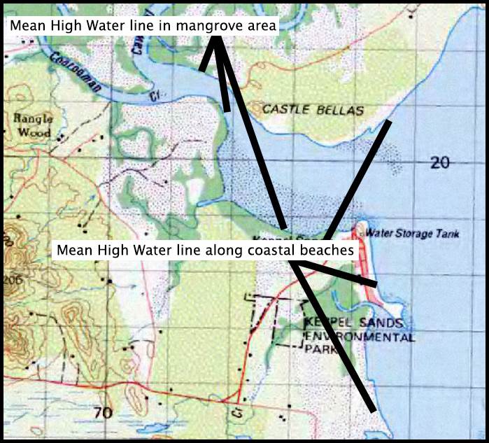
Section of 1: 100 000 scale NTMS showing the depiction of mean high water in areas of coastal beach and mangroves.
Coastlines at Mean Low Water, Mean High Water, and Lowest Astronomical Tide
Madden stated in his paper that Mean High Water (MHW) was chosen as the most appropriate waterline to depict the coastline on the 1: 100 000 scale map series so that the blue line on these maps depicted the location of mean high water except where mangroves occurred. A mangrove area was defined as the land upon which the mangrove is situated between the low and high water lines. In the case of an area of mangroves a broken blue line was shown on the seaward edge of the mangrove symbol and this line was stated to be an approximation of the coastline. This decision was made to simplify the cartographic presentation of mangroves as well as to overcome the difficulty of identifying the coastline when it was located within a stand of mangroves which could be misleading to the map user. On open beaches mean high water was a recognisable blue line on the map, whilst within mangroves it was not, please see map above showing examples of this depiction. On topographic maps this decision meant that the mean high water line thus became the defacto zero contour. Decisions about the depiction of Mean Low Water (MLW) were a little more complex.
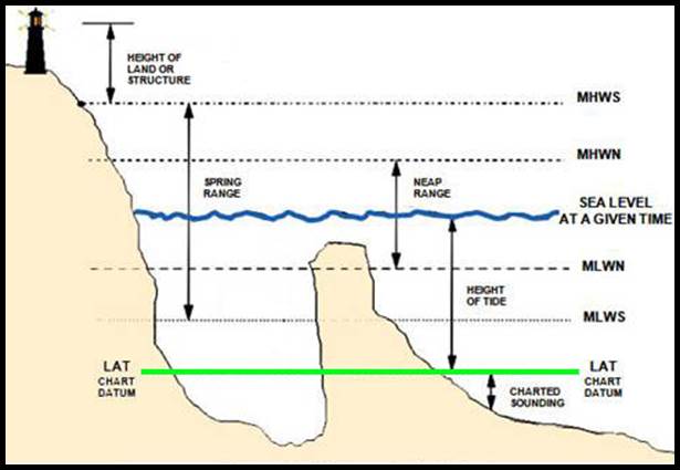
Diagrammatic relationship of tides; noting that older Australian charts used the chart datum of the mean of the lowest low water spring (MLWS).
Australia had participated in the 1958 United Nations First Conference on the Law of the Sea, in Geneva. This Conference as part of its work, produced the Convention on the Continental Shelf. This conference then led to the Conventions on the Territorial Sea and the Contiguous Zone and on the Continental Shelf. Australia became a signatory to these Conventions in 1963. In so doing, Australia undertook to learn as much as possible about the nature and extent of its own continental shelf. This knowledge was required so that this region could be delineated and any exploitation adequately controlled. The bathymetric mapping of the continental shelf by National mapping began in 1971 as is described in Bathymetric Mapping – Natmap’s Unfinished Program.
Today the Law of the Sea is a body of international rules and principles developed to regulate ocean space, as reflected in the 1982 United Nations Convention on the Law of the Sea (UNCLOS). Australia participated in all three United Nations conferences on the Law of the Sea (1958, 1960 and 1973-82) and became party to UNCLOS in 1994. Under Article 76 of UNCLOS Australia had the right to make a submission to the Commission on the Limits of the Continental Shelf (CLCS) to delineate the outer limits of these areas of extended continental shelf and define the limits of Australia's jurisdiction over the seabed and subsoil beyond 200 nautical miles (370 kilometres).
Critical to the determination of all maritime boundaries under UNCLOS, was the determination of the Territorial Sea Baseline (TSB) around Australia and its remote offshore territories. Essentially, the Territorial Sea Baseline was the line of low water along the coastline. However, the United Nations Convention on the Law of the Sea allowed for the Territorial Sea Baseline to jump across bays, rivers and between islands, as well as along heavily indented areas of coastline, under certain circumstances. Further, Article 5 of United Nations Convention on the Law of the Sea defined the baseline as the low water line along the coast as marked on large scale charts officially recognised by the coastal State. Low water was not defined, however, and Australia decided to use Lowest Astronomical Tide (LAT) as this was the datum that was already being used on hydrographic charts.
Lowest Astronomical Tide (LAT) was defined as the lowest tide level which could be predicted to occur under average meteorological and any combination of astronomical conditions. Finding Lowest Astronomical Tide along Australia’s extensive coastline was just impractical so a best estimate would be initially based on charting, large scale topographic maps, satellite imagery, and other sources. In the interim, however, mean low water would be used as the indicator for baseline determination for territorial boundary purposes and maps with these baselines were prepared for negotiations between the Commonwealth and the States. From Natmap’s Bathymetric mapping program and the specialised tide based aerial photography program, the position of Lowest Astronomical Tide was gradually revised, as appropriate.
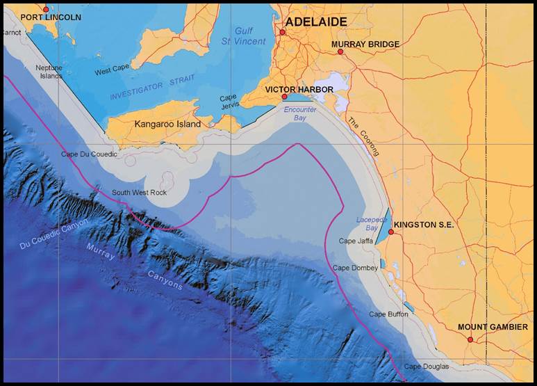
Section of map showing examples of the Territorial Sea Baseline along normal and indented coasts and bays (courtesy Geoscience Australia).
As already mentioned, the Territorial Sea Baseline corresponded with the position of Lowest Astronomical Tide along the Australian coastline, including the coasts of islands or low tide elevations. Low tide elevations were defined as naturally formed areas of land surrounded by and above water at low tide but submerged at high tide, provided they were wholly or partly within 12 nautical miles of the coast. Where the coastline was deeply indented and cut into, or where there was a fringe of islands along the coast in its immediate vicinity, a straight line between specified or discrete points on the water line could be used to define the baseline. A straight line between specified or discrete points on the water line could also be used to define the baseline across the natural entrance points of bays or rivers. Any waters then on the landward side of a baseline were thus internal waters for the purposes of international law.
The Tide Controlled Coastal Aerial Photography Program
The aerial photography program from which the maps of the NTMS were derived was planned according to season and map priorities. In coastal areas acquiring this photography could be difficult enough due to weather let alone acquisition at specific tide times. Additionally, in contrast to the mapping photography, the coastal photography required only a few frames at a larger scale and the film emulsion used for the mapping photography was not suitable for coastline determination. It was also foreseen that in regions having beaches with a shallow gradient and/or where the permanent tide gauge network was too sparse, Natmap would need to undertake additional surveys and observations to elicit the necessary tidal data. A separate, specialised program of aerial photography using Natmap’s existing aerial cameras with an infrared film and photography acquisition time meeting the tidal conditions, was thus commenced as described below.
Aerial Film
The aerial film selected was Kodak’s 2424 Black & White Infrared, then available in 70 and 230 millimetre frame formats. This film was sensitive to ultraviolet, visible, and infrared radiation to approximately 900nm with maximum sensitivity from 760 to 880nm (nanometres or nm is 10-9 metres). Infrared radiation (light) does not penetrate water, to any great degree, so it appeared black in the photos. The terrain and vegetation reflected light and so features could be seen to enable the plotting of the land-water interface. Please refer to the illustrative example below showing the same area acquired with colour film and infrared film. As it was desirable to confine the exposure to the far red and infrared regions of the spectrum a Wild 600 nm (WRATTEN Filter No. 25 equivalent) or light-red filter was employed to absorb all of the blue portion of the visible spectrum and nearly all the green. The result was that the land/water boundary was clearly evident on the photography and haze effects found in coastal areas were negated (the use of a yellow filter was also trialled but the red filter was found to produce better results).
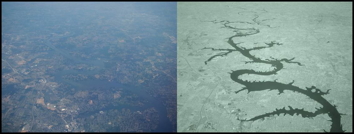
Same area acquired with colour film and infrared film.
Aerial photography for mapping was essentially only governed by cloudless skies and the sun being high enough not to cast long shadows or no shadows at all. This usually gave a morning and afternoon window of opportunity. For coastal photography within those two nominal windows the tide had to be right as well – not easy even with two (usually) tides a day!
The standard mapping aerial photography specifications were thus relaxed. As acquiring the photography at or around Mean Low Water was the most important requirement more flexibility was permitted with the light conditions ensuring only good, even light; so not too early or too late in the day. To some extent photography acquisition became a judgement call by the Party Leader.
Depending on the aerial camera used, flying heights ranged up to 10 000 feet ASL, the limit without the need for crew to be on oxygen.

Rockwell Aero Commander 500 Shrike, VH-PWO, contracted from Executive Air West,
used for coastal photography by Natmap in 1976 and 1977 in Western Australia; pilot Max Cooper (XNATMAP photograph).
Aerial Cameras
Natmap used both the Swiss Wild RC9 and RC10 aerial camera with their superwide angle lens and 9 inch x 9 inch (23cm x 23cm) film format. The operational camera was floor mounted in a contracted, twin engine, high wing aircraft like a Shrike Commander. The table below lists the year along with the aerial camera(s) used and the nominal photoscale(s) of the acquired coastal photography. All photography was captured with a nominal 60% forward overlap to provide stereoscopic coverage for water line delineation.
|
Year |
Photoscale |
Camera |
Serial No. |
|
1971 |
1: 35 000 |
RC9 |
616 |
|
1972 |
1: 35 000 |
RC9 & RC10 |
616 & 1336 |
|
1973 |
1: 23-52 000 |
RC9 |
374 & 616 |
|
1974 |
1: 34 000 |
RC9 |
616 |
|
1975 |
1: 26 000 |
RC10 |
1336 |
|
1976 |
1: 35 000 |
RC9 |
373 |
|
1977 |
1: 35 000 |
RC10 |
1336 |
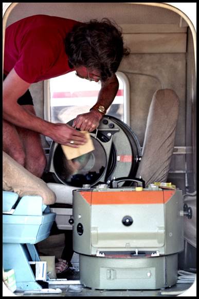
Wild RC10 aerial camera in Rockwell Shrike VH-PWO in 1977, being prepared for photographic mission by Bob Smith (XNATMAP photograph).
The smaller film format, 70 millimetre, Swedish Hasselblad camera was also used with the photoscale dependant on flying height. The Hasselblad was generally floor mounted in a contracted, high wing, single engine aircraft like a Cessna. The only currently recorded Hasselblad photography was acquired at Mean High Water in 1972 over the coastal reaches shown on the SD52-10 Medusa Banks and SD52-11 Port Keats, 1: 250 000 scale map sheets, which span the Western Australia – Northern Territory Border. The Medusa Banks photography was acquired from an altitude of 5 000 feet resulting in an approximate photoscale of 1: 35 000 while the Port Keats photography was acquired from an altitude of 10 000 feet resulting in an approximate photoscale of 1: 70 000.
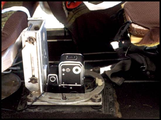
Hasselblad camera, mounted in a Natmap designed and constructed floor mount to enable its near vertical orientation during photography operations (XNATMAP photograph).
Tide Prediction
Tidal data on the Australian coast was integrated into a homogeneous system with the introduction of the Australian Height Datum (AHD) in 1971. The then tide gauge network was predominately along the south east coast leaving the north and north west region with relatively few permanent tide gauges. Thus the harmonic tidal constituents needed for tide prediction were variable and based upon limited periods of tide gauge observation. The tidal data published in the Australian National Tide Tables was essentially accepted as the best information available for predicting tides on the Australian coast.
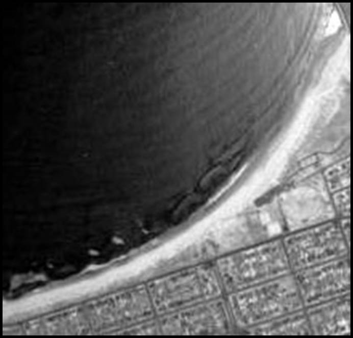
Section of RC10 aerial photograph of beach near Newcastle NSW, acquired in 1974 at Mean Low Water,
showing dry sand (bright tones), wet sand, breaking waves and deep water (dark tones).
To obtain all of the 37 tidal harmonic constituents, the tides at a location required observation for a minimum of a year. Locations which had a longer series of data typically used harmonic constants based on multiple years. The 37 tidal harmonic constituents comprised 10 diurnal, 12 semidiurnal, 5 long term and 10 for shallow water (diurnal means daily and semidiurnal means approximately every half day). It was, however, possible to isolate the seven main harmonic constituents responsible for the tidal conditions at a location and these are tabled below. These seven major factors were enough to provide a suitably accurate estimate of tidal conditions.
|
Main Tidal Harmonic Constituents |
|||
|
Name of Tidal Constituent |
Cause |
Time Scale |
Symbol |
|
Principal lunar semidiurnal |
Gravitational effect of the Moon |
12 hrs 25 min |
M2 |
|
Principal solar semidiurnal |
Gravitational effect of the Sun |
12 hrs 00 min |
S2 |
|
Larger lunar elliptic semidiurnal |
Variation in the Moon's orbital speed due to its elliptical orbit |
12 hrs 39 min |
N2 |
|
Luni-solar Declinational semidiurnal |
Declinational effect of the Moon and Sun, respectively |
11hrs 58 min |
K2 |
|
Luni-solar Declinational diurnal |
Effect of Moon's Declination |
23 hrs 56 min |
K1 |
|
Principal lunar Declinational diurnal |
Diurnal inequality of Moon's Declination. |
25 hrs 49 min |
O1 |
|
Principal solar Declinational diurnal |
Sun's Declination |
24 hrs 04 min |
P1 |
Up to 1976, predictions for tide condition were mainly precomputed in the office prior to field flying operations. During 1976 and 1977 portable programmable calculators were available which allowed onsite tidal prediction and the planning of the coastal flight times. As is discussed below, for a good part of the 1977 operations, the planning of flight times was more reliant on real time tidal observation due to the sparsity of permanent tide gauges and the significant tidal variations in the survey region.
Field Operations
The tide controlled coastal aerial photography acquisition program, commenced in 1970 within the newly established Map Completion Section, mentioned above. In the first couple of years the testing of films and film/camera filter combinations was undertaken and an operational procedure established. Ground truth testing facilitated the gaining of expertise in the interpretation of the water line on the aerial photographs. In these early years the tidal based photography was only acquired when the map areas were undergoing map completion checks prior to publication.
Aerial operations were necessarily based upon tidal predictions, which predetermined the most suitable times for photographic sorties. The duration of flying operations centred around the time of the required tide height being captured on the photography.
Ultimately, it was also determined that in addition to the aerial photography, the field party needed to have observers on the ground. Depending on the region these observers may only have been required to record the tidal readings on the nearest tide post(s) so that any local current or wind effect on the tide during photography could be determined. In other places these observers or temporary tide gauges were deployed well before the aircraft operations were to commence to determine additional tidal data so that more reliable tide times could be determined.

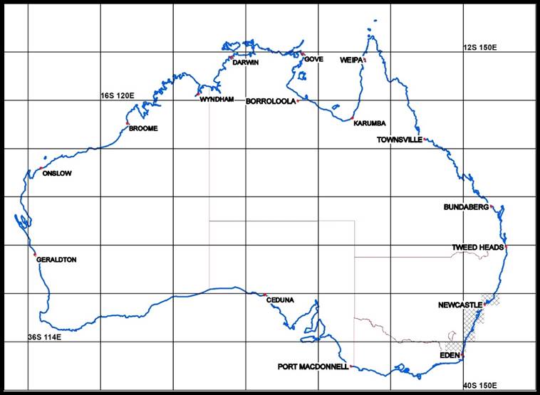
Map showing areas where coastal photography was acquired at Mean High Water during 1971.
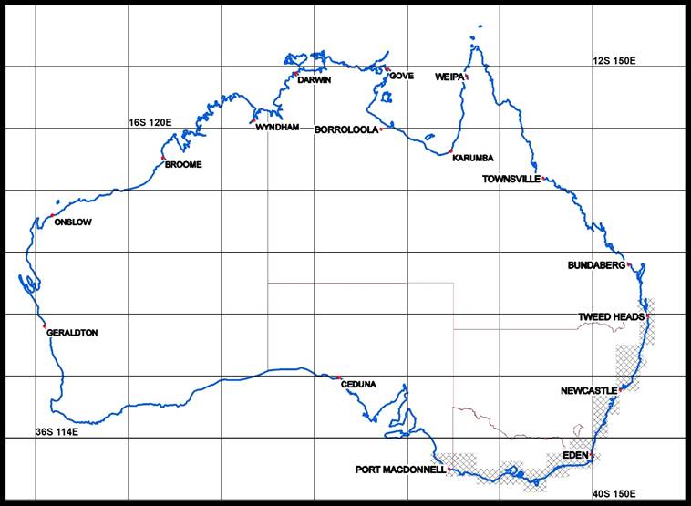
In 1971 a specific program of tide controlled coastal photography was instigated. The program initially acquired photography so as to define the sections of coastline, as indicated by Mean High Water, where gradually shelving beaches and a low hinterland would require the airborne component be supported by additional ground survey. The first section of coastline acquired was in the Proserpine and Mackay areas of Queensland, in 1971. In 1972, photography of coastal stretches from Broome to Kalbarri, Western Australia, and in the Bowen and Rockhampton areas of Queensland, was acquired. The first photography captured at Mean Low Water was acquired along the New South Wales coast between Newcastle and Eden.
The 1973 program captured extensive northern coastal stretches, at Mean High Water, from Bundaberg in Queensland around to Derby in Western Australia. As the steep rocky coastline of the Kimberley region had only a vertical tidal movement, the area was excluded. As part of the 1973 program a Piper PA-23-250 Aztec D (VH-PRB) was used by John Manning, David Bruce, Reg Helmore and others during October and November for the photography of the coastal sector from Broome to Gove.
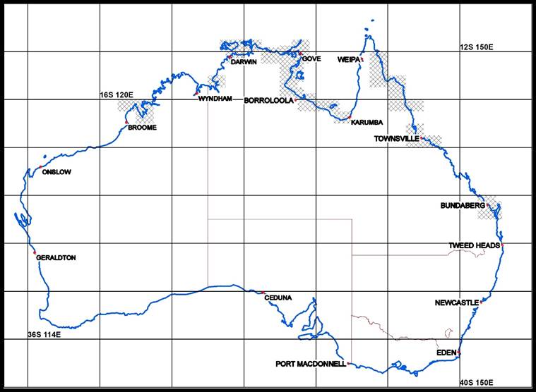
Map showing areas where coastal photography was acquired at Mean High Water during 1973.
Operations for 1974/75 were run out of the Canberra office under Surveyor Gordon Homes. In preparation for the 1975 photography program of the Victorian coast, short period tidal observations were made at Cape Conran, Ninety Mile Beach, Wilsons Promontory, Apollo Bay, Port Campbell and Portland. The 1974 program captured missing coastal sections from the 1973 program between Townsville, Queensland and Darwin in the Northern Territory, with some sections of the coast reacquired closer to the time of the high water tide. The New South Wales coastal section around Eden and from Newcastle to Tweed Heads was acquired at Mean Low Water.
From the preceding years’ work, proclamations of coastal baselines, with accompanying maps, were drafted and baselines for southern New South Wales and south eastern Tasmania were finally gazetted on 31 October 1974, by the Attorney General's Department. New boundaries were calculated for oil leases affected by the Australian-Indonesian border in the Timor Sea.
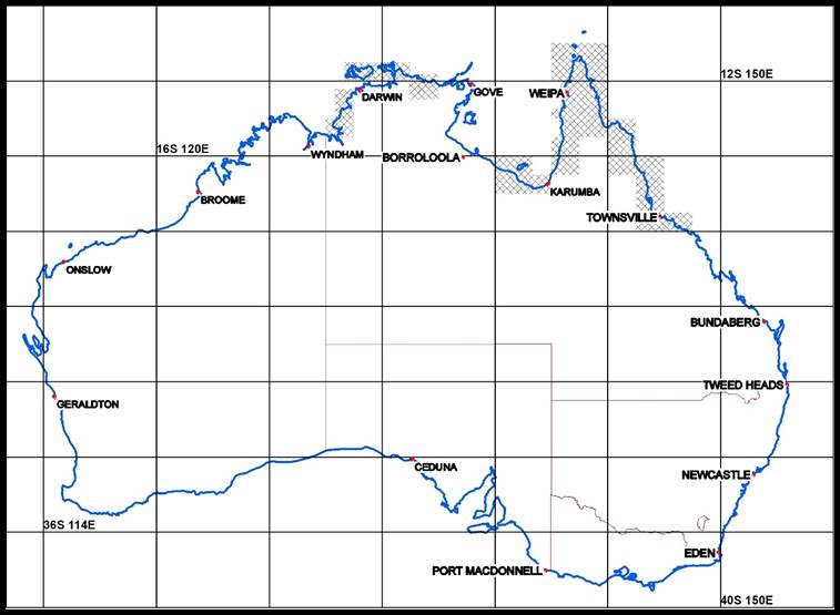
Maps showing areas where coastal photography was acquired at Mean Low Water during 1975.
From February to April 1975, tide controlled photography to determine the line of Mean Low Water was acquired of the entire coast of Victoria, extending from Eden just over the border in New South Wales to Port Macdonnell just over the border in South Australia. Some sections of the New South Wales coast, photographed in 1974, were reacquired when it was found that cloud and shadows had seriously affected the previous photography.
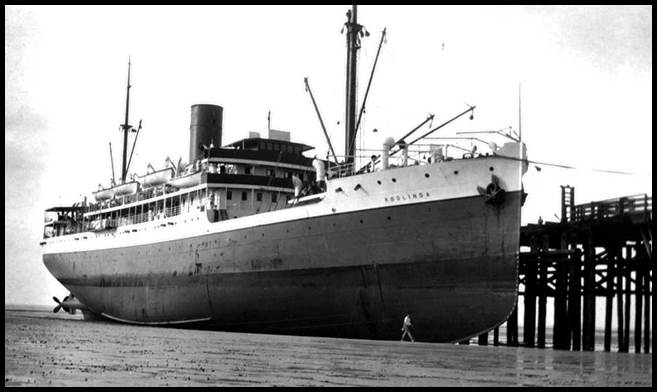
Circa late 1930s photograph of the coastal steamer MV Koolinda sitting on the mud beside the pier at Broome (courtesy seabooks.net/redbill/images).
In 1976 and 1977 the coastal photography program was undertaken by the Melbourne office. During this time the more complex areas of the north west coast were to be captured on film. The complexity of the task was due not only to the remoteness of the region, but also to the sparse permanent tide gauge installations in that part of Australia and the large tidal variations signified by a nominal 10 metre difference between low and high tide at Broome. Please refer to the photograph above.
Between 16 November and 16 December the 1976 photography program of the coastline at Mean High Water and Mean Low Water was completed from Broome to Geraldton, comprising the areas of Roebuck Bay, 80 Mile Beach, Karratha, Dampier, Hedland, Onslow, Barrow Island, Tryal Rocks, Exmouth, Carnarvon, North West Cape and Jurien Bay. Offshore features also photographed were Bernier, Dorre and Dirk Hartog islands, the Houtman Abrolhus, Bedout Island and Rowley Shoals.
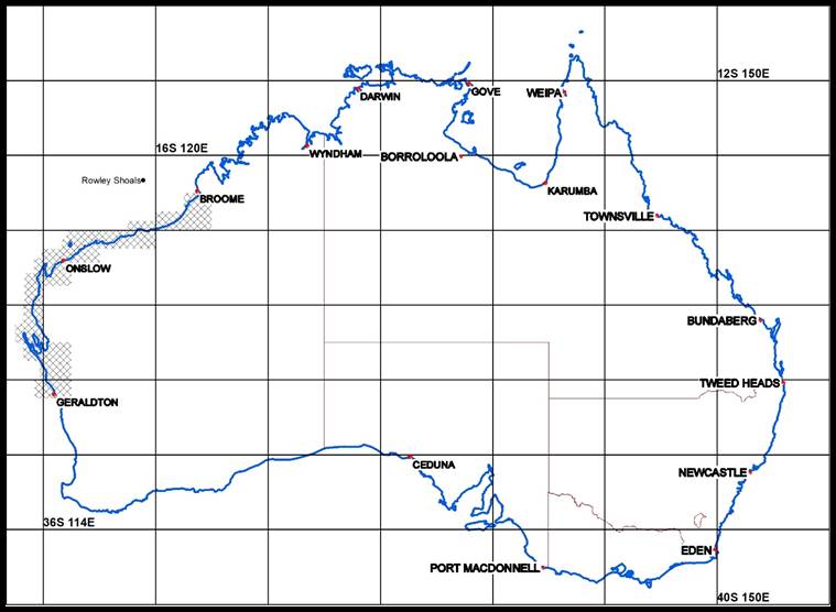
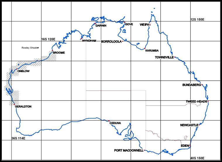
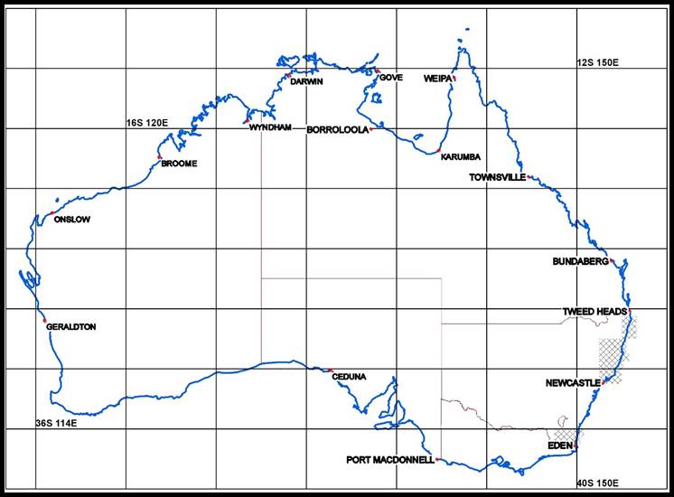
Maps showing areas where coastal photography was acquired at (left) Mean High Water and (right) Mean Low Water during 1976.
The 1976 Nat Map field party comprised Party Leaders Andrew Turk (initially) and Paul Wise who completed the whole field season. Photography line navigator was Bill Stuchbery and the Wild RC9 camera operator was Graeme Lawrence. Real time tidal data was recorded by Mick Lloyd, Andrew Hatfield, Steve Pinwill, Bob Goldsworthy and Hayden Reynolds. Oz Ertok joined the party as the electronics technician. The aerial survey camera was mounted in a chartered Shrike Commander 500S (VH-PWO) piloted by Max Cooper.
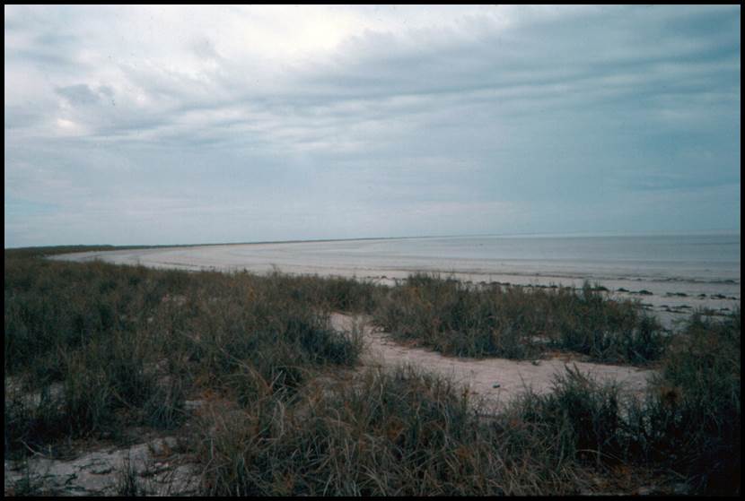
After completing the section from Broome down the 80 Mile Beach to about Cape Keraudren and before operations were shifted to Port Hedland the offshore features of Rowley Shoals needed to be captured. Rowley Shoals was some 300 kilometres off Broome and according to the hydrographic charts and Notes to Mariners at low tide there were areas that fall dry. Mermaid, Clerke and Imperieuse reefs were the three atolls that comprised the shoals. Refer map below.
Map showing Rowley Shoals off Broome, consisting of Mermaid, Clerke and Imperieuse Reefs.
With the possibility of dry areas it was important that such areas be photographed at both high and low altitudes. Transit time, some 2 hours each way, and the fact that the time of Mean Low or High Water might be somewhat in error due to the Shoals’ distance from the coast, where the tide harmonics for calculation had been derived, had to be considered as well as time to loiter. The plan In the end involved flying out at 5 000 feet from which height it was safe to navigate and see the shoals on arrival. In the area, climb to 10 000 feet for the photoruns (two north south runs per atoll) then descend to wave-top to fly around for 35mm oblique photos out of the copilot’s window which could be safely opened in flight. On 9 November 1976, the Shoals’ were photographed at Mean High Water. At low level, the sea could be seen gently breaking all around an area of grey wet sand, scattered with a few black lumps of coral rock. As there was no indication of any area(s) being permanently dry, island status could not be conferred. Later on 12 November 1976 the Shoals’ were photographed at Mean Low Water.
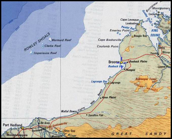
Section of 80 Mile Beach west of the Sandfire Roadhouse on the Great Northern Highway, selected for gradient survey (XNATMAP photograph).
Beach gradient surveys were recorded at Broome’s Cable Beach and on the 80 Mile Beach west of the Sandfire Roadhouse on the Great Northern Highway. At Onslow, further beach gradient surveys were conducted as well as successful sea water penetration tests. These tests determined the depth to which the infrared radiation penetrated the sea waters of this area.
|
|
|
|
Broome’s Cable Beach in foreground and pier in background (XNATMAP photograph). |
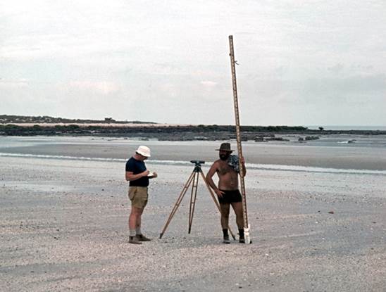
Gradient survey of Broome’s Cable Beach; (L-R) Paul Wise and Mick Lloyd (XNATMAP photograph). |
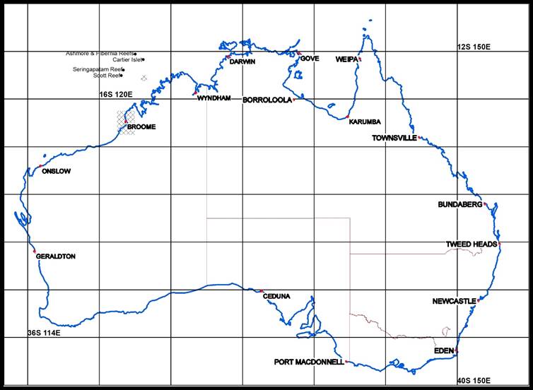
The 1977 coastal photography program was undertaken between 28 May and 15 July. The coast between Broome and Darwin, comprising the areas Lagrange, Broome, Pender, Lacepede Islands, Cape Leveque, Yampi, One Arm Point, King Sound, Disaster Bay, Valentine Island, Derby, Wyndham, Cambridge Gulf, Medusa Banks, Port Keats, Adele Island, Beagle Reef, Mavis Reef, Victoria River, Cape Bernier, Geebung, Darwin, Fog Bay and Pearce Point, was acquired at Mean High Water. On 4 June 1977, the offshore features (refer map below) of Scott Reef, Seringapatam Reef and Browse Island and 14 June 1977, Ashmore Reef, Hibernia Reef, Cartier Islet, were acquired at Mean Low Water, as were the coastal sections of the SE51-06 Broome and SE51-10 Lagrange 1: 250 000 scale map sheets. Much of the steep rocky Kimberley coast was again excluded from the program.
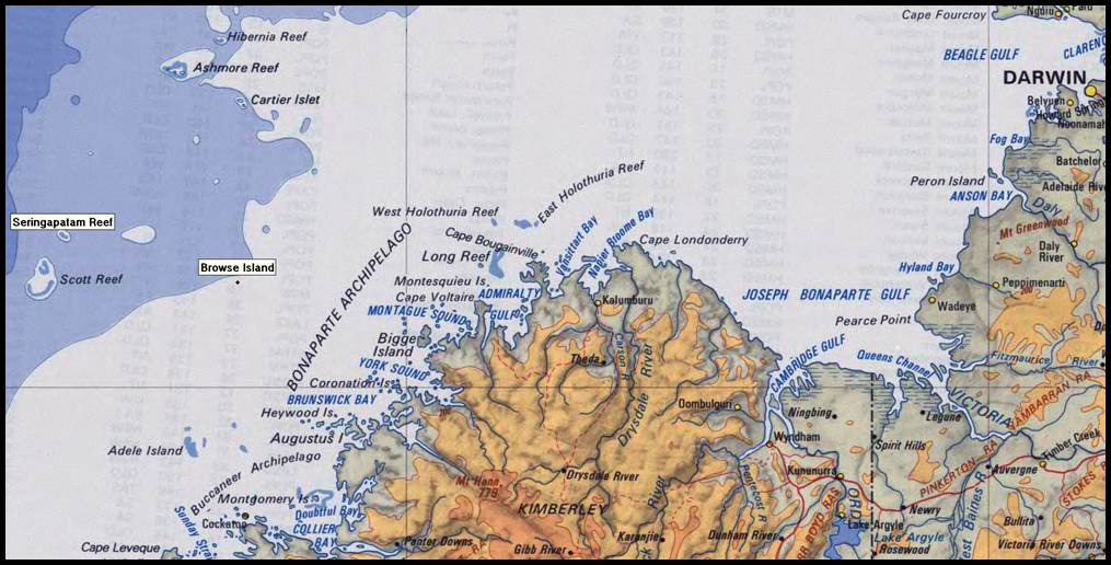
Map showing the offshore features of Browse Island, Scott Reef, Seringapatam Reef, Cartier Islet, Ashmore Reef and Hibernia Reef.
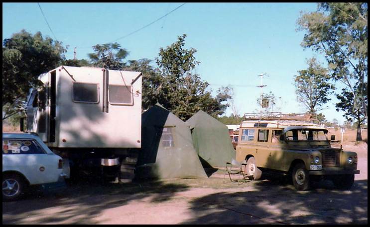
1977 camp at Wyndham with Natmap mobile office caravan (courtesy Bill Stuchbery).
The 1977 Natmap field party comprised Party Leader Rom Vassil who was later replaced by Carl McMaster. Photography line navigators and Wild RC9 camera operators included Ed Burke, Joe McRae, Bob Smith and Bill Stuchbery. Real time tidal data was recorded by Mick Lloyd, Steve Pinwill, Bob Goldsworthy, Reg Kearns and Ted Rollo. As in 1976, the aerial survey camera was mounted in a chartered Shrike Commander 500S (VH-PWO), piloted initially by Jack Marshall and later Max Cooper.
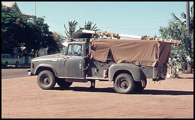
Tide poles being transported on roof rack of International C1300 in 1976 (XNATMAP photograph).
As mentioned above, in this region of Australia only limited tidal information was available from official sources so observation camps in the operational area were established. At these camps, homemade tide poles were emplaced and round the clock observations made to enable the tidal cycle to be established. (Two tide poles had been made in late 1975 by the field staff, in the then basement workshop of the Rialto Building. The poles were solid timber about 3 metres long, painted white with length annotations in black. The tide poles had been carried during the 1976 season but where not required).
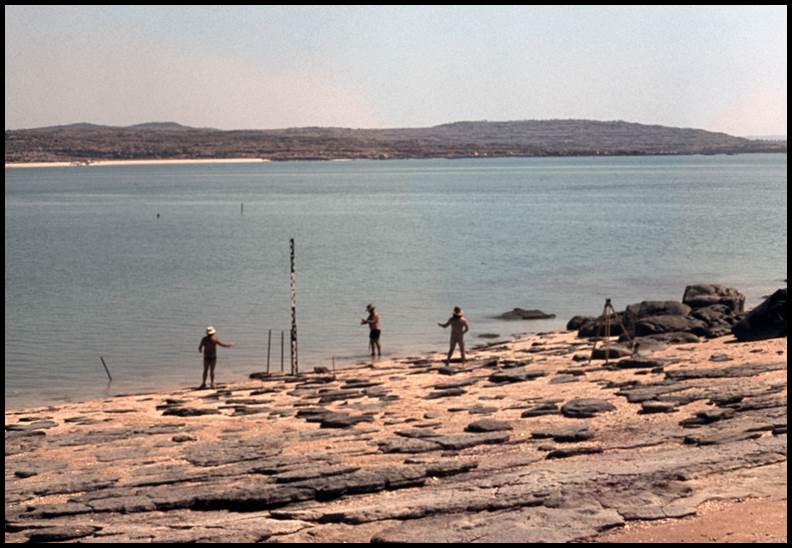
Erecting a tide pole; (L-R) Reg Kearns, Mick Lloyd and Steve Pinwill (XNATMAP photograph).
Because of the tidal range both tide poles were emplaced and the tidal information radioed to the flight crew enabling the flight lines to be planned. One such camp was at One Arm Point at the western entrance to King Sound, where the aircraft was able to land at the nearby sand strip. It was found that near Cape Bernier in the Kimberly there almost zero tide yet not far east and west the tidal difference was over 12 metres.
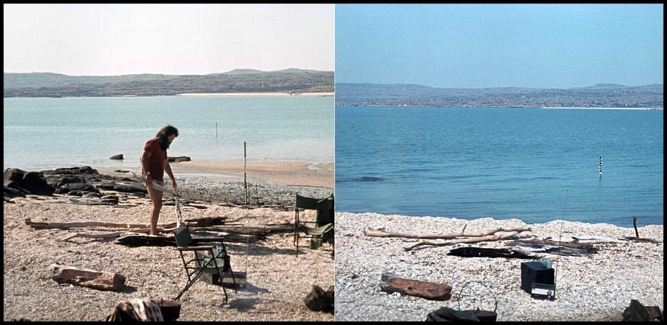
Comparative photographs showing the two tide pole arrangement and the extent of tidal activity with Steve Pinwill (XNATMAP photographs).
Records showed that the last tide controlled aerial photography was acquired in 1978, at Mean High Water, in the SI53-01 Nuyts 1: 250 000 scale map sheet area of South Australia.
Map showing areas where coastal photography was acquired at Mean High Water during 1978.
The Outcome
As well as defining a blue line on a coastal map sheet, the coastal delineation by aerial photography program was a precursor to the declaration of Australia's Exclusive Economic Zone (EEZ) on 1 August 1994. The zone extends from 12 to 200 nautical miles (22 to 370 kilometres) from the coastline of Australia and its external territories, except where a maritime delimitation agreement exists with another state like Timor and Papua New Guinea. The map below shows the extent of the EEZ in Australia’s region.
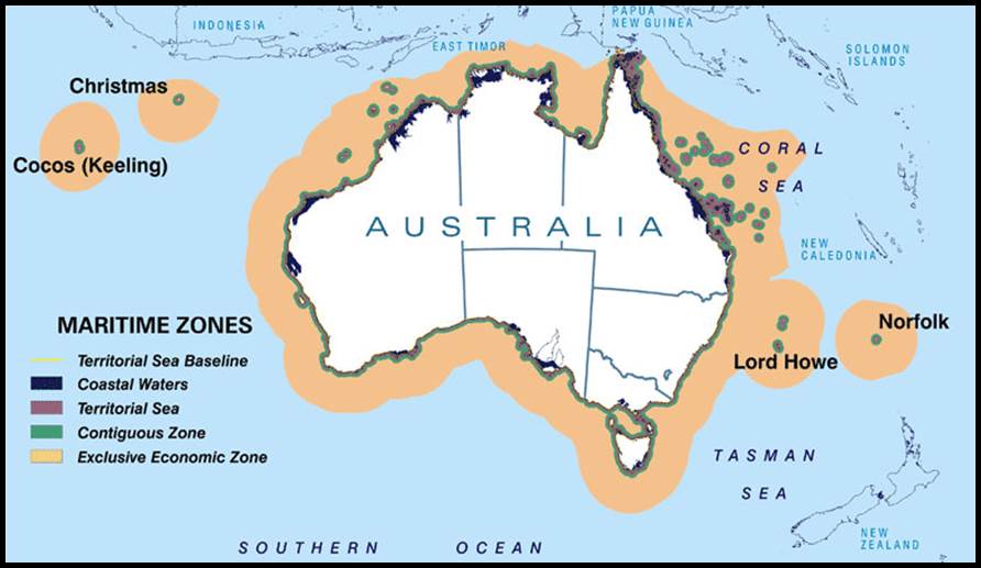
Section of map showing Australia’s Maritime Zones (courtesy Geoscience Australia).
Acknowledgement
Thanks to Bill Stuchbery for extracting information on the 1976 and 1977 field seasons from his diaries.
by Paul Wise, 2022
Sources
Geoscience Australia (2022), Maritime Boundary Definitions.
Geoscience Australia (2022), Computing Australia's Maritime Boundaries.
Madden, John Donal (1977), Coastline Delineation by Aerial Photography, first presented 48th ANZAAS Conference, Melbourne, 1977, republished The Australian Surveyor, 1978, Vol.29, No.2, pp.76-82.
McLean, Lawrence William (2021), Gordon Morris Homes.
Watson, Charles W and Wise, Paul J (2022), Bathymetric Mapping – Natmap’s Unfinished Program.