Nat Map Training Notes

1.1.1 The direct measurement of distance with a steel band is referred to as "chaining”, from the use of the original Günter’s chain of 100 links. Modern steel bands are generally about 3.18mm wide and 0.25mm thick. The length now being used within the Division is 50 metres. The bands are graduated with stamped brass rivets or sleeves.

1.2 Plumbob

1.2.1 This is used for testing the verticality of beacon poles, transferring to ground the end marks of steel bands, setting the theodolite over fixed points and step chaining.

1.2.2 To hold the plumbob cord on the tape, the cord and tape are pinched together by the thumb and forefinger, at the points shown by the arrows in Figure 1.2.2.

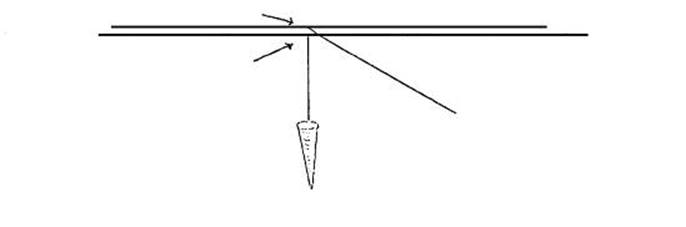
Figure 1.2.2.

1.2.3 The two extreme positions likely to be encountered when using the plumbob to transfer the position on the tape to a ground point, or vice versa, are:-

(a) shoulder height. This is the limit without losing accuracy;

(b) peg height.

1.2.4 When using the plumbob, there will be slight movement of the bob, due to vibrations from the tape, wind, etc. This movement can be reduced to a minimum by gently tapping the ground with the point of the plumbob.

1.2.5 When the line of sight from the theodolite to a point is obstructed, it is possible to use the plumbob as a target. In order to minimise the error due to the movement of the plumbob, the string should be held as close as possible to the top of the plumbob. The point of the plumbob should be kept as close as possible to the point being plumbed. The correct method of holding the plumbob is shown in Figure 1.2.5.

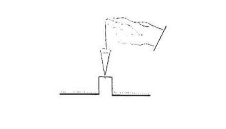
Figure 1.2.5.

1.2.6 In order to mark a point with the plumbob, the tip of the bob should be about 13mm above the ground, and when the order to mark is given, the assistant settles the plumbob and a clearly defined hole is made with the point. If the ground is too hard for the point to mark, the plumbob is kept in the position shown in Fig. 1.2.6 until a chaining arrow is inserted.

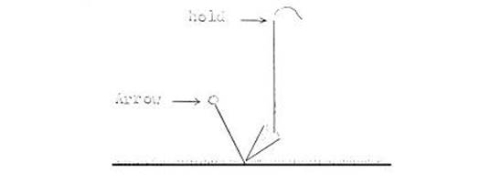
Figure 1.2.6.

1.3 Care of the tape

1.3.1 When unrolling the band, 1 assistant takes the free end of the tape and walks slowly forward, while the other assistant holds the arrow on which the cross revolves, or the strap of the reel, so that the band comes off freely and easily, without jerks. The man at the cross or reel end also sees that the band does come off too quickly, and that it does not get caught on obstacles. As his end of the band comes in sight, he warns the man at the other end to be prepared to stop, at, the same time preparing to give a little at his end, in case of a sudden jerk. When the end of the band is reached, he gives the signal to stop, and both men lay the ends of the band on the ground, ready to start work.

1.3.2 In rolling up, the band is first laid out straight on the ground and one end is fastened to the cross or reel. The man working the latter, now starts to walk slowly towards the other end of the band, at the same time winding it up. In doing this he sees that it is not caught on any obstruction and is wound firmly and tightly without any sudden jerks taking place. When the end is reached, it is fastened to the cross or reel by means of a strap or leather lace.

Although most steel tapes used for surveying will withstand a direct tension of 36 Kilograms (about 80 lbs.) it is very easy to break them by misuse.

When a tape is allowed to lie on the ground, unless it is kept extended so that there is no slack it has a tendency to form small loops like that shown in Fig. 1.3.3. When tension is later applied, the loops become smaller either it jumps out straight or the tape breaks, as shown. If a tuft of grass or any object is caught by the loop, the tape almost always breaks or at least develops a permanent "kink". To avoid this, the tape must be handled so that no slack can occur. For measurements of less than a full tape length, the tape should be kept on the reel. It should be reeled out to the necessary length, and reeled in as soon as possible. The assistant, who handles the reel, must reel in any slack that might occur between the two assistants, while the tape is being handled. For measurements greater than the tape length, when the tape is off the reel, the tape should be kept fully extended in a straight line along the direction of measurements. When it is to be moved, it must be dragged from one end only.

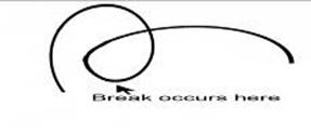
Figure 1.3.3.

If it is necessary to raise the tape off the ground, the two assistants must lift the tape simultaneously and keep it in tension between them. Except for this operation, the rear assistant must not touch the tape while it is being moved. If he picks up the rear end, and moves forward faster than the other assistant le will form a "U" in the tape, which usually causes a loop to form when the tape is pulled taut. This may break the tape.

1.3.4 When the end of the measurement is reached, where a less-than-tape-length measurement is required, the assistant must not pull in the tape hand over hand as this creates a pile of loose tape on the ground. Instead, he must do one of three things:-

(i) Carry the end of the tape, beyond the point, lay it on the ground, and walk back.

(ii) Reel in the tape, the requisite amount.

(iii) Take in the tape, forming figure-eight loops hanging from the hand. Each length of tape must be laid in the hand flat on the previous length and never allowed to change. Later, to extend the tape, lay it out carefully as he walks forward, by releasing one loop at a time. This method requires care and practise and should not be attempted until the required skill has been obtained by practise.

1.3.5 No vehicle should be allowed to run over the tape. Only in the case where the tape is across a smoothly paved street can a pneumatic tyred vehicle pass over the tape without damaging it. The tape must be held flat, and tightly pressed against the street surface by the two assistants.

1.3.6 When a tape is wet, it should be carefully cleaned, one oiled immediately after use.

1.3.7 In general, it is well to remember that a tape is easily damaged but, with care and thought, damage seldom occurs, keeping the following in mind:-

(a) Keep the chain straight. If, for any reason it is necessary to pull it back do so from the end, rather than let it lie in a series of loops at an intermediate point from which it is pulled.

(b) If pulling the chain around a corner see that it is pulled around a curve of large radius, and have an assistant watching it to see that the sleeves do not catch in a splinter or a piece of barbed wire or anything else which might break the chain.

(c) If the chain is caught do not attempt to free it by jerking but go back and release it where it happens to be caught.

(d) In running out a Box Tape from its case see that it runs out tangentially and is not bent back where it leaves the case. The tape should always be kept bright and clean.

If it gets wet, dry it at once, and if it becomes muddy, wash the mud away with clean water then dry the tape. It should never be wound up into the case when wet, but while drying it should be hung in a series of wide loops, which will allow it to dry quickly.

If it becomes dirty or rusty it should cleaned with kerosene, oil, or some non-abrasive such as "Brasso".

1.4 Step chaining

1.4.1 Measurements are carried forward by holding the tape in a horizontal position, and the plumb line is used by either or at times, by both assistants for projecting from tape to ground. Figure 1.4.1. shows an example of "Step chaining".

Figure 1.4.1.

1.4.2 It requires some practise to judge when the tape is horizontal. The best way is to pull sufficiently to eliminate sag and hold the stretched tape so that the angle between it and the plumb line is a right angle. It is impossible to judge horizontality from the uphill end of the tape.

1.4.3 In step chaining the length of the step will depend upon the angle of slope, and should not be so long that the height of the plumbed end above the ground exceeds 1.5 metres.

1.4.4 It should be noted that holding one end of a 50metre tape 1 metre above or below the true horizontal line will cause an error in the result of 8mm. Hence the need for a very close approximation to the level line, at the instant of plumbing.

1.5 Slope Chaining

1.5.1 The tape is held on a slope and the angle of slope read so that the measurements can be reduced to the horizontal.

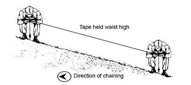
1.5.2 The chain may be held at any convenient height at both ends however it is usual practise to hold waist high, the rear assistant reading the slope.

1.5.3 For slopes up to 4° the Abney Level (See 1.6.) is used to read the angle of slope. For slopes above 4° a theodolite should be used to read the vertical or slope angle. The theodolite is set accurately over the chained point, and the angle of slope read, to the assistants hand as he releases the plumbob at the "mark" signal.

1.6 The Abney Level

1.6.1 This is one of the popular instruments of the surveyor's kit. It is not a precise instrument by any means, angles of slope are read to within two minutes, in the larger size, and to within ten minutes in the smaller size. There is no magnification in the sighting tube through which the bubble and target are viewed at the one time. Below is shown, the method of using the Abney Level for chaining. A 4° slope is being read which is the allowable limit for the Abney Level.

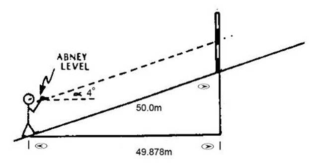
Figure 1.6.1(a)

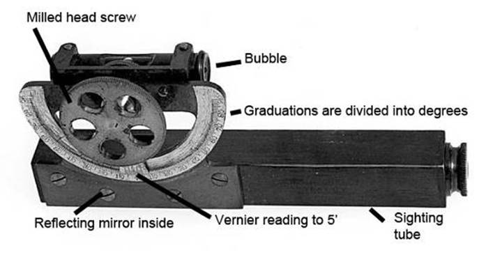
Figure 1.6.1(b)

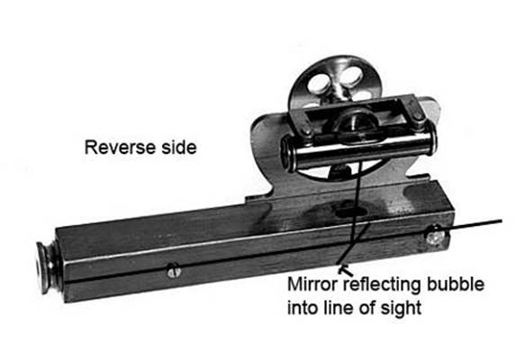
Figure 1.6.1(c)

The graduated circle is divided into degrees, and the vernier to read to 5 minutes = 11 divisions of graduated circle divided into 12. Reading either side of index to 5¢.

1.6.2 Adjustment of the Abney Level

By taking the mean of back & fore sights. Two points of different elevation are selected, and the vertical angle between them is observed from both.

The angle of elevation observed from the lower station should equal the angle of depression from the higher. If not, the mean is the correct reading and the instrument is made to record this by the adjusting screws on the level.

Alternative to (b), the index error can be used :-

If the reciprocal observation gives 15° elevation and 17° depression, the index error is half the difference, i.e. 1° to be deducted from all depression angles and added to all elevation angles.

The following is probably a better method of recording and using, an Abney Level correction:-

With a theodolite determine the altitude of a well defined object some 500 metres away. Set this angle on the Abney Level, sight on the object with the Abney Level. Observe, carefully, where the sighting mark "cuts" the bubble reflection. It may be half or quarter way down from the top, etc. In future determinations of slope bring the bubble to this same position, relative to the sighting mark. When continuous use of the Abney Level is being made, it should be tested, as described, every 2 or 3-days.

1.7 Errors in chaining

1.7.1 Even experienced assistants have difficulty in preventing the tape and the plumbobs from moving, during measurements. The error from this source is, between 1:5,000 and 1:10,000. Variations in tension of 2.27kilogrammes (about 5 lb) introduce an error of 1:10,000 with a tape of average cross section, 50 metres long, and supported at the ends. Temperature may introduce an error of up to 1:5,000 so that, all in all, this type of measurement has an accuracy seldom better than 1:2,500. Using spring balance handles will improve the accuracy to 1:3,000. With temperature correction, as well, an accuracy of 1:5,000 can be attained.

1.7.2 If more accurate results are required then special equipment is necessary.

1.7.3 A distinction should be made between errors and blunders. Errors result from such things as:-

Incorrect alignment of the chain.

Temperature variations.

Tension variations.

Tape not straight.

Blunders are usually due to:-.

Miscounting of chain lengths.

Misreading the chain.

Erroneous booking.

Misplacement of a chainage point.

1.8 Use of Spring Balance and Thermometer

1.8.1 It should be noted that a 50 metre tape will expand or contract 1mm for every 2°C change in temperature, or 8mm for every 15° C. It is very difficult to read an exact temperature of the tape.

In general, the thermometer should be held as close to the tape as possible, while taping is taking place. The ideal situation would be to have the thermometer clipped onto the band, with the bulb in contact with the steel.

1.8.2 The spring balance is simply attached to one and of the band and tension is applied, until the tension, at which the tape has been standardised, is reached. This is generally about 3.630 kilograms (about 8 lb) to 4.600 kilograms (about 10 lbs), when using the 50 metre band for chaining.

Tension should not be applied quickly, but as a gentle pull, applied by the leading assistant; this will reduce jerking, etc.

1.9 Clearing lines for chaining

1.9.1 Prior to commencing chaining, the line should be cleared of all obstacles which may tangle or bend the tape. Grass, scrub and trees, should be cut down as low as possible, and where chaining is to take place, with the tape resting on the ground, the line should be scraped free of all vegetation, rocks, etc. The principal problem in clearing vegetation from a survey line is maintaining a straight line.

If this is done, the effort involved is kept to a minimum, and work progresses more rapidly and systematically. Quite often, large trees have been felled only to find later that they were well off line. It is far better to take some trouble to locate the correct line. This is best done by using "sighting sticks" or "boning rods".

The first stick is set on the required line by theodolite or compass, at some convenient distance from the station. The axeman can then walk "on line" by looking back and aligning himself with this stick, and the theodolite. Before he loses sight of the back mark, in this case, the theodolite, the axeman should cut another bush stick, an inch or so, in diameter, driving it into the ground, on line with the previous marks. He then maintains direction by aligning himself with the two closest marks. This process is carried on for as far as necessary. Shorter sticks are used when clearing over a ridge; and longer ones when crossing a depression. If carefully executed, straight lines can be maintained for considerable distances, say about 1 kilometre, with an error of about half a metre, depending on the terrain.

1.10 Reading the chain

1.10.1 Steel bands, now in use in the Division of National Mapping comprise a 50 metre steel section, marked with brass studs each metre. Attached to the zero end of the band is a leader 1 metre plus long. The leader is graduated to millimetres.

1.10.2 In order to measure an uneven distance, the leader is held roughly over the forward station, by the forward assistant. The rear assistant then holds the nearest graduation on the band over the previous chainage mark. At the "read' signal given by the rear assistant, the reading on the "leader" is noted by the forward assistant, and the rear assistant reads, the whole metre on the band. To minimise the possibility of misreading, the two assistants now change position, and the procedure is repeated. See Figure 1.10.2.

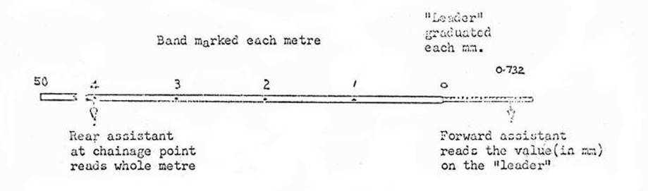
Figure 1.10.2.

Rear assistant reads 04.000 metres.

Forward assistant reads 0.732 "

Distance 04.732 metres

1.11 Third Order Traversing

1.11.1 Theodolite and chain traverse

This is the method by which cadastral survey work is carried out, and boundaries of properties, measured and marked, or re-established, on the ground.

In mapping, 1st and 2nd order traverses are now carried out with electronic distance measuring equipment, taking the place of the chain. However, there is still a need for traversing of 3rd or 4th order standard. The latter is often a short connection to a photo reference point, etc., where a spring balance and accurate slope corrections are a needless refinement.

It is envisaged that traversing similar to the third order traverses would be required to connect mapping control points to distant satellite stations, or short traverses to get mapping control into timbered flat, terrain, unsuitable for electronic measuring equipment.

1.12 Accuracy Standards for Third Order Traversing

1.12.1 Error between traverse control points and adjacent control

The traverse control points should be determined with sufficient accuracy so that, after adjustment, it will be unlikely that the computed distance between a 3rd order control point and any adjacent 3rd or higher order, control point, will be in error by more than 1 part in 5,000.

1.12.2 Errors of standardisation, and between adjoining stations of the traverse.

The probable error of standardisation of the field tape should not exceed 1 part in 50,000 (i.e. an error of 1mm in the 50 metre tape) and the linear distance between adjoining stations on the same traverse, should be within 1 part in 25,000.

1.12.3 Angular error

The angles of the traverse should be measured to a uniform degree of accuracy, and the maximum misclosure at an azimuth station, or trigonometrical station should not be greater than 12 Ö n seconds where "n" is the number of traverse stations between azimuth control, thus, with 25 stations the misclosure should be 12Ö25 = 60 seconds or less. The angular adjustment per station should never exceed 5 seconds and seldom exceed 3 seconds.

1.12.4 Heights carried through traverse

Heights carried through the traverse by vertical angles should be correct to 1.5 metres after closure adjustments have been made.

1.12.5 Terminal control and azimuth control

Third order traverses must start and finish at third or higher order control points; and at intervals of 20 to 30 stations along the traverse; at permanently marked stations an azimuth check should be made. The probable error of this azimuth observation should not exceed 5².

Azimuth observations should also be made at junction stations. At first sight, the above standards may seem rather high, but, provided the chain is standardised accurately, they should present no problem to experienced personnel. Angles will usually be read with a Wild T2 theodolite, and the chaining will normally be along the ground, not in catenary or suspension.

It will be found that the initial linear surround is likely to be within 1 part in 12,000 to 15,000 or better.

1.13 Marking the Traverse

1.13.1 Permanently marked stations

These should be established at intervals of not more than 3kms along the traverse, with an average distance of about 1.5 kms. Two reference marks, one of which could be a reference tree, should be established at each station.

1.13.2 Marking of intermediate stations

These stations should be marked by temporary wooden pegs, about 25mm x 25mm x 200mm

1.14 Location

1.14.1 Access

Roads and fences will usually greatly expedite the work, if one proceeds in the right direction, and if the road does not carry heavy traffic or raise dust, to hinder the work. The traverse should run just off the road edge, and about half to one metre from the fence.

1.15 Traversing Party

1.15.1 Make up of party

If trained personnel are available and an efficient, economical party is required in fairly open country, the four man party is suggested.

(a) A theodolite observer who reads and records angle and bearings in a field book.

(b) A senior assistant who holds the back end of the chain, and records field notes in respect to chainage measurements, Abney Level slopes, and laid distances, references, etc. Notes taken in this second field book will require transcription later on, into the field book which records the angular work.

(c) An assistant who takes the front end of the chain, applies the required tension, and usually reads the "reader", for any references required.

(d) Another assistant nominated as the "axeman", who clears the line, and sets the pickets. If a vehicle can be taken near the line, and there is little cutting, the axeman may be able to bring the vehicle along.

However, there are many variations, even in the 4 man party. If the clearing is heavy, the axeman and assistant may both cut, and the senior assistant may take the front one of the chain, where he does the booking, leaving the theodolite observer on the back end of the chain.

Or the observer may do the booking of both angles and chainage, with the senior assistant setting pickets, driving the vehicle forward, and taking the front end of the chain. This will require a certain amount of walking by the senior assistant.

Again, in easy country, a 3 man party (axeman-picket setter; assistant; theodolite observer) can make good progress.

A 5 man party, if available, may also be economically employed, (2 men clearing, picket, setting and bringing on transport; one senior assistant; one assistant; one theodolite observer.

A party of 2 experienced, energetic men (observer and assistant) will also make good progress where there is no cutting to be done.

All the above work presupposes that the traverse stations are selected and located, as the traverse proceeds, and that chaining is not done in catenary, but along the ground. Reference marks on trees or corner posts should be observed and measured as the work proceeds, but it must be decided whether it is economical to emplace concrete blocks, and concrete reference marks, at selected stations as the traverse is run, or at a later stage, this depends on the going, and the availability of personnel.

1.16 Distance between Stations

1.16.1 This depends on the terrain, and on the observing conditions. Along straight roads or fences, in gently undulating country, 1.5 km legs are possible, in conditions of good observing. In hilly, heavily timbered country, where a road is being traversed, it may be difficult to see 100metres, on occasions, and special care in centring the instrument becomes essential, to hold the azimuth.

On open plains, in hot weather, it may be necessary to read the angles in the early morning, and late afternoon, though the chaining can be carried out during the day. These, decisions must be made by the party leader, depending on conditions prevailing at the time. Work will usually be expedited by the use of the longest legs which can be observed; if someone has to be sent to show up the forward or back pickets for the observer, much time will be lost.

Assistants should be trained to keep slightly off line, except when they are actually laying the chain, and so allow the theodolite observer to read his directions, once the forward picket is plumbed. With long straights, under open conditions, where the forward picket cannot be seen with the unaided eye, it is the responsibility of the rear assistant, and the observer to see that the chain is laid on line, or within 0.30m. Generally, in flattish, open timbered, country, legs from 350 to 500 metres will give best observing conditions and results.

1.17 Pickets or Targets

1.17.1 Pickets

Traversing in bush country is likely to be carried out by observing to pickets cut from saplings or branches, as work proceeds.

Such pickets may be from 1 to 2 metres long, and 50mm to 75mm in diameter, sharpened at the bottom for driving into the ground, and with a "step" cut in the side 300mm to 450mm from the bottom, to assist such driving. The top 100mm to 150mm, should he cut to a straight four-sided, tapering point, or to a four-sided squared top with 25mm wide sides.

A 40mm x 50mm rectangular, or 40mm square, piece of white folded paper placed carefully, and centrally on the pointed picket, leaving about 13mm to 25mm showing, makes a good sight, however distance and visibility govern the size.

On occasions, the point may not be seen and the paper will then need to be bisected; it should therefore be carefully centred by the picket setter. If, for some reason (such as stock in paddocks or along roads) the squared top picket is adopted, a white papered top may assist visibility, and a strip of paper about 150mm x 50mm wrapped near the top makes a good sight for bisection. Spitting on the last few millimetres, of the strip of paper, when wrapping it around the pickets, is a crude but effective method of holding it.

A pointed picket is an extremely dangerous object to be left standing in open grazing country, on a road, or wherever animals could impale themselves. They must not be left standing.

In bushy country, it may be advisable to use pickets about as high as the telescope of the theodolite. This will ensure that the observer will always see his back picket after moving forward. Along roads, or in open country, the observer will probably prefer to use pickets about 1 metre high, over which he can set his instrument. The temporary wooden pegs, under each picket are often more safely hit in by the observer, after he has set his instrument over the picket. To counteract accidental bumps to the pickets before the instrument is set up, the pickets should be accurately plumbed by the picket setter, and a match (or hole made by the plumbob point) left to indicate the plumbed position.

1.17.2 Targets

Special traversing equipment is made by several firms. Instead of sighting to a picket, a metal target in black and white is used, which may be screwed to the theodolite tripod, and levelled with footscrews. For quickest results, the theodolite tripod and target tripods are interchangeable. The tripods are set up firmly, the targets levelled, and angles read with the theodolite the head of which is then unscrewed and transferred to one of the tripods from which the levelled target has been removed.

It will be realised that with four sets of tripods, three targets and one theodolite, a continuous series of steps can be undertaken with no hold-up. Work of the highest quality is possible with such sets.

1.18 Field Chaining

1.18.1 Chains

Most third order chaining has been done with the 300 foot steel band. However, future chaining will be done with metric bands, probably the 50 metre band. The characteristics of the 50 metre bands currently in use within the Division are:-

Width 3mm

Thickness 0.05mm

Weight, approx. 0.680kg (1 metre = 0.013607kg.)

These characteristics agree closely with those of the 300 foot band previously in use: ‑

Width 1/8² (0.125")

Thickness 1/50" (0.02")

Weight approx. 2.51b. (1 ft = 0.0083 lb.)

It should be mentioned at this stage that the 15lb tension applied to the 300 foot band of approximately the same characteristics will probably be too great for the much shorter 50 metre band, and would tend to pull the assistant "off balance". A tension of 4.600kg (10.14lb) will probably be satisfactory for the 50 metre band; however this could be the subject for further investigation.

1.18.2 Chaining with the 50 metre band

Chaining in catenary, i.e. with the tape fully suspended, or with one, two, or three supports, is the recognised method of accurate chaining. The number of men required, in a party engaged on such measuring, and the effect of wind, (nearly always prevalent in the open areas of Australia) on the suspended steel band, are the drawbacks to this method.

If the ground chaining surface was perfectly flat, such as along a straight bitumen road, along the rail of a railway line, or on a claypan, the tape could be laid on the surface; with the correct tension applied, each end could then be marked by a fine scratch or pencil line. However such conditions are exceptional, and even under conditions with little or no undergrowth, it will be found that rocks, grass tufts, etc., prevent the band from lying flat enough to give an accurate horizontal distance. Also with the band completely along the surface, accurate temperatures are much harder to obtain.

Thus for normal field conditions with a small party it can be considered impractical to either chain in full catenary or completely along the ground, therefore it is necessary to adopt a compromise between the two methods.

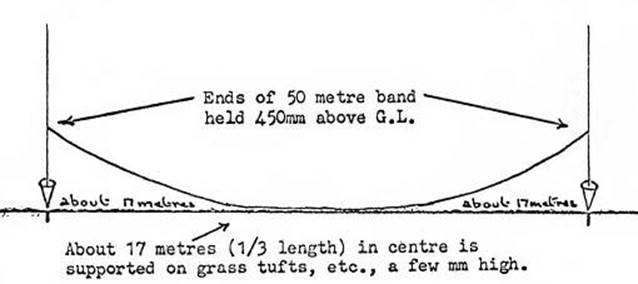
Figure 1.18.2(a)

Each end of the band is held 450mm (approx. 18" or knee high) above the general level of the ground, or of the vegetation which supports the tape. A "pull" of 4.600 kg (approx 10 lb) is applied to one end of the band. Under this tension the effect is for about one third of the band at each end to be elevated with the central third supported a few millimetres above the ground on low bushes, grass tufts, etc. This method of chaining counteracts slight ground irregularities and obviates excessive low clearing. See figure 1.18.2(a).

When using this method, a standard "sag" correction for each 50 metres is determined at the time of standardization before the chaining task is undertaken. See paragraph, "Check against standardized steel band."

If high grass undergrowth supports the chain at a fairly regular height, the senior assistant will estimate this general supporting height and have the band held at the normal 450mm above this general height.

In all cases temperatures should be taken at the general height of the band, not with the thermometer lying on the ground, as this yields a highly inaccurate temperature for a band held as described.

Use of plumbobs

The skill needed to accurately use the above method is all in the use of the plumbobs, and can only be acquired by plenty of practise. Sixteen ounce plumbobs of the "conical" type, which enables easier viewing of the mark from directly above, should be used in preference to the "pear shaped" type.

The rear assistant has the most difficult task, he should double the surplus plumbob string through the brass loop in the end of the band, holding this string in the palm of the right hand, and using his right leg as a lever to keep his right arm and hand steady, (the reverse for a left-handed person, in all cases). The left hand should keep the plumbob string both at the right, height and against the outer edge of the brass loop on the end of the band. 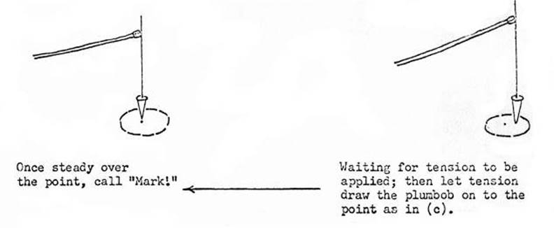While waiting for the forward assistant to take up the tension, the plumbob's swing should be continually "dampened" by tapping its point on the ground, a few millimetres to the right of the mark. As the forward assistant takes up the tension on the spring balance, the rear assistant allows this tension to draw his plumbob directly over the mark; once there and steady, he calls loudly "Mark" If this system is practised, and adopted, it will obviate the "tug of war" so often seen with inexperienced assistants. See Figures, 1.18.2(b) and 1.18.2(c).

Figures, 1.18.2(c) and 1.18.2(b)

Check against standardized band

One 50 metre band should be properly standardized and held solely for the purpose of standardizing field bands. Ideally, this band should be of "invar"; also all steel bands should have the same characteristics. A suitable tension for field use should be adopted for standardization; this saves the calculation of a correction for tension and the need to apply it to every length laid in the field.

The field bands should be checked against the standard band in two ways, i.e.:‑

(a) On a perfectly flat surface, in the shade, lay out an exact 50 metres with the standardised band. Use the correct tension and apply a temperature correction, if necessary.

Each field band is checked against this base at the same tension, and the temperature recorded. The difference in measurement gives the error of that particular 50 metre band at that temperature. This difference would only be used to correct any 50 metre length which may be chained along the ground.

(b) Using the exact method to be employed in the field task, a full 50 metre length is laid out against the exact 50 metre base, the temperature is taken and the difference in measurement is noted. This difference will be a set correction covering "sag", "tension", and "error in length" for each 50 metre length laid at a corresponding temperature. Thus only temperature corrections need to be calculated for each length laid in the field. It is unlikely that many lengths will be laid completely along the ground, however it is a simple matter to make the check outlined in (a) above in case some lengths are more conveniently laid on the ground.

The usual procedure in laying the chain is briefly:-

(a) The forward assistant pulls the chain ahead, taking care that it does not go under bushes or rock snags, and counting his paces, to stop approximately at the correct distance. He will have to get used to the pace-metre ratio.

(b) The chain is straightened by "throwing up" each end, holding it lightly taut, and throwing a wave motion along the tape. Two hands should be used, one hand holding the end by balance or plumbob cord, the other stretched as far along the tape as possible to help in "throwing up" the tape, in the small wave motion mentioned. Do not jerk the chain sharply.

(c) With chain straight and free, the front assistant puts on the 4.600 kgs (about 10lbs) tension to obtain an approximate position for placing the arrow. He eases off the tension, and with his heel kicks away the grass, etc., to make a clear spot for the plumbob mark.

(d) He again applies the 4.600 kgs tension, holds his plumbob string right at the end of the chain, and lowers the plumbob to about 25 to 50 mm above the ground. The rear assistant holds his plumbob string at the rear end of the chain, with the plumbob point 12mm or less, above where the arrow enters the ground. Both assistants are holding the chain ends 450mm above the general supporting height of the tape.

(e) When the tape is steady, it is kept thus for 3 or 4 seconds, and the front assistant drops his plumbob to make a light mark on the cleared surface. Then he eases off the tension. If either assistant is dissatisfied with the laying of the chain it must be done again.

The front assistant carefully inserts an arrow, slanting and at right angles to the line being traversed, in the centre of the plumbob mark. This completes the laying of one length of the chain, the procedure being repeated as many times as necessary. The above method of chaining gives a distance, for each length of chain laid, that is slightly short of the length of the chain; each 50 metre length will need to be corrected by the standard correction covering "sag", "tension", and "error in length" that was ascertained in the check against the standardised steel band. In addition each length laid will be subject to the temperature correction for the prevailing temperature.

1.19 Field Chaining – Odd Lengths

At the end of a traverse leg there is usually some odd length to be measured. The method is for the front assistant to hold his end of the chain at the peg, whereupon the rear assistant pulls the chain back until he, the rear assistant, is holding on a brass mark. The front assistant then reads the odd length, on the reader, at his end of the chain when tension is applied. On arrival at the peg, the rear assistant should be shown, and should check this intercept, and should report the value of the brass mark that he plumbed. (See Figure 1.10.2) Roller-grips for odd lengths are very desirable, and should always be used, if available. In all chaining, the body should be used to take the tension by resting the elbow just above the bent knees, or if the chain support is higher, by pressing the elbows or wrists hard against the body.

1.20 Corrections to chained distances

The following are brief notes on the corrections which affect third order traversing.

1.20.1 Standardisation

Normally, one tape has been standardised by an authority such as a State Lands Department for a small fee. A sample certificate can be seen here. Before commencing a task, field tapes have been checked against this tape as explained in 1.18.2.

1.20.2 Slope correction, and use of the Abney Level

This is the most frequent, and usually the largest correction applied in chaining; its purpose being to reduce measurements which have been taken on sloping ground, to horizontal measurements.

These slopes, or angles of elevation or depression, are generally read with an Abney Level; the rear assistant reading the same height (eye height) on the forward assistant. There is a probable error of 5 minutes with such a reading. This is not a cumulative error, but has a serious effect on corrections for slope over 4°. For these the theodolite should always be used.

In hilly country, where large slopes are common, consideration must also be given to chaining in catenary, so that accurate slopes may be determined.

Slope corrections are calculated by multiplying the versine of the slope angle, by the measured length. These corrections are always minus, whether slopes are elevation or depression.

A table of slope corrections for every 5¢ from 0° 25' to 5°, and covering the distances in use, is the quickest way to reduce slope distances, in normal country.

Natural versine values for every minute are listed in Chambers Mathematical Tables, and some slide-rules incorporate a versine scale.

1.20.3 Temperature correction

Since steel expands when heated, a chain standardized at 15°C (59°F) and used in the field at 32°(approx. 90°F) will be too long; requiring a plus correction, for temperature, for all measurements made with it.

A coefficient of expansion for steel chains may be taken 0.000 0113 per 1°C (0.000.0063 per 1°F). A table showing the correction for temperature and length can be seen here.

The formula for temperature correction is:-

Ct = 0.000 0113 L (T-To)

where Ct = Temperature correction.

0.000 0113 = co-efficient of expansion of steel per 1 C.

L = Measured length.

To = Temperature of standardization of to

T = Temperature of tape in field, in °C

It is difficult to obtain accurate temperatures in the field; temperatures can be as much as 1° to 5°C in error, usually too high. If conditions are normal, it is not necessary to read a temperature at every length laid, and a reading every fourth tape laying should suffice.

Care should be taken to see that such temperatures are read at the height of the chain; that is, when chaining across foliage which supports the chain, at about 300 mm above the ground, the chaining thermometer should be laid horizontally, and at that height; not laid on the ground, which on a hot day with a light breeze, might give an error, of 5°C, or more, too high.

If the thermometer is placed at the correct height, then the chain laid, and the slope read and booked, enough time should have elapsed for the thermometer to have moved to the correct temperature.

Inver bands are sometimes used. This is an alloy of nickel and steel, with a very low coefficient of expansion, approximately 1/30th that of steel. If standardisation is made close to the prevailing field temperatures, then temperature corrections may be disregarded with these bands.

1.20.4 Tension correction

This is a correction which should seldom be necessary. If the tape is standardised at a correction suitable for field use, and used at the same tension, no correction is necessary. The formula for computing variation in tension is:-

Cp = { (P – Po) L} / AE

where Cp = The correction per distance L, in metres.

P = Applied tension in Kilograms.

Po = Tension of tape at standardisation, in Kilograms

A = Cross-sectional area, in square cm's.

E = Young’s Modulus of elasticity of the steel in the tape

taken at 2,003,750 Kilograms per square cm.

1.20.5 Sag correction formula

Where W = Weight of tape in kilograms per metre.

L = Length of unsupported tape, in metres.

P = Tension in kilograms.

Sag correction Cs = { W² * L³ } / {24 * P² }

When a tape is supported in equidistant spans, this formula becomes:-

Sag correction Cs = n [ { W² * L³ } / {24 * P² } ]

where n = Number of equal spans into which tape is divided.

L = Length of each span in metres.

With slopes over 10°, a further factor is introduced due to the deformation of the catenary.

Formula for Sag correction on slope = sag correction on level x Cos² slope angle.

To calculate sag using SI units this article is useful.

This will rarely be necessary. Since sag reduces the length, the measured distance is longer than the actual distance, so correction “negative”.

1.20.6 Sea level Correction

This will rarely be applied in the field. Generally mean height can be used for the traverse, the sea level factor is set on a computing machine, and all measured distances are multiplied, in turn, to give a sea level distance.

1.21 Summary of chaining Corrections and Errors

1.21.1 Standardisation

If incorrectly standardised, the one tape will give an accumulating error of the one sign. Tapes should be carefully standardised, under good conditions.

1.21.2 Errors in slope reading

Where slopes are read with the theodolite, errors should be negligible. When the Abney Level is used, and is checked every few days, against the theodolite, errors of reading should cancel out, in lightly undulating country.

1.21.3 Temperature

The main source of error likely to occur, is from placing the thermometer at a different height from the tape; usually too near the ground which will make the readings too high.

A general mean of conditions, to which the tape is subjected, should also be chosen for the thermometer; that it is not protected from the wind, or put in the shade, unless the tape is under such conditions. The thermometer should be carried vertically so that the mercury column is not shaken apart, but laid horizontally, at the mean height of the tape, and given a chance to settle before reading. Much time can be lost, and little extra accuracy gained, through elaborate temperature reading, but reasonable care must be taken. Temperature errors are likely to be cumulative, on the one day, under similar weather conditions, and usually too high.

1.21.4 Tension

If the spring balance is reading incorrectly, this will give a cumulative error. It is advisable to check all balances, by lifting a known weight, or by pulling against the other balances.

1.21.5 Sag

In uneven country, sag must be watched carefully, and it will be decided whether to chain in catenary. Sag errors will rarely occur in easy, flattish, terrain. They are cumulative.

1.21.6 Alignment

Keep alignment within 150 to 300mm, and no appreciable error will result. Alignment is more easily maintained by the rear assistant, who should direct the front assistant on line before laying the chain.

1.22 Algebraic signs of errors using a single tape

When speaking of chaining errors:-

“+” means an error which tends to make a distance measured longer than it actually is, on the ground; thus the correction to the measured distance is MINUS.

“-“ means an error which tends to make a distance measured longer than it actually is, on the ground; thus the correction to the measured distance is PLUS.

The following list of errors shows the accumulating effect.

	Error	Accumulating effect
a	Standardization	All plus or all minus
b	Slope	Plus & minus
c	Temperature	Plus usually
d	Tension	All plus or all minus
e	Sag	All plus
f	Alignment	All plus
g	Height of tape	Plus & minus

1.23 Errors of a full chain

Every distance laid must be entered, at once, in the field notes. Recourse should never be made to the counting of arrows, or to both assistants trying to remember the number of full lengths laid. The dropping of one full length is the most frequent source of gross error in chaining. Occasional wooden tally pegs, (about every ¾ kilometre) are useful, in case an arrow should be accidently knocked out, on a long traverse leg. This can prevent returning to the beginning of the leg.

1.24 Check measurements

These should be made if possible; more especially on large surrounds, to pick up gross errors. They may be made later, or by a second pair of assistants following the traverse party, and a lower order of accuracy is possible. Slopes and tensions are read, but not temperatures and other refinements.

1.25 Angular measurements

Angular measurements will normally be made with the Wild T2 theodolite, or similar instrument.

1.25.1 Horizontal Angles

The mean of 2 rounds is adopted as the observed angle at each station; each round consists of a face left and a face right pointing, on the distant stations. Settings are approximately:-

FL 000° 00’ 30" returning to the RO on 180° 00’ 30" approximately.

FR 270° 05’ 30" returning to the RO on 090° 05’ 30" approximately.

The RO should always be the backsight, and the difference between the pointings should not exceed 10 Seconds.

1.25.2 Vertical angles

Heights are carried through the traverse by vertical angles. Two pointings, a face right, and a face left, are read from each station, to both backsight and foresight, and always that order. The heights of the instrument, and of both targets are recorded in the field book, as each is measured.

1.26 The Surveyors Level

The function of the surveyors level, more commonly termed simply, the level, is to establish a horizontal line of sight, or nearly so. In its simplest form, it consists of a telescope with a defined line of sight and a spirit level tube to enable this line of sight to be set in a horizontal plane.

The modern levels which are likely to be met with, are:‑

The Tilting Level, and

The Automatic Level.

An almost obsolescent level is the Dumpy Level which had the telescope body fixed at 90° to the vertical spindle.

1.26.1 The Tilting Level

The main features of the telescopes incorporated in Surveyors Levels are that they have low magnification and a small field of view, suitable for accurate sighting over the short distances required. The diaphragm normally has a central horizontal and vertical wire; in addition two horizontal "stadia" wires are set equidistant, above and below the central horizontal wire. They are normally set so that the distance read on the staff between these two wires (known as the "intercept" or "S") is one hundredth of the distance between the level and the staff when the line of sight is horizontal. Ratios, other than one to one hundred can be ordered from the maker, if required.

The spirit level attached to the telescope is similar to those used on theodolites, and provision is also made for its adjustment in a similar manner.

To operate the instrument, the telescope with its attached level tube can be levelled by a finely pitched screw - called the tilting screw - independently of the vertical axis, and in consequence the line of collimation is not in general at right angles to the vertical axis. In using these instruments, the axis is set only approximately vertical with the three footscrews with reference to a circular bubble. Before reading the staff, the bubble in the main level tube which is attached to the, telescope, is centred exactly by means of the tilting screw.

In better instruments this is done by bringing the ends of a split bubble into coincidence. The bubble ends and the staff are viewed through the telescope at the same time, and coincidence of the bubble ends is made at the instant of reading the staff. Mirrors to read the bubble are used instead of the split bubble on low priced instruments.

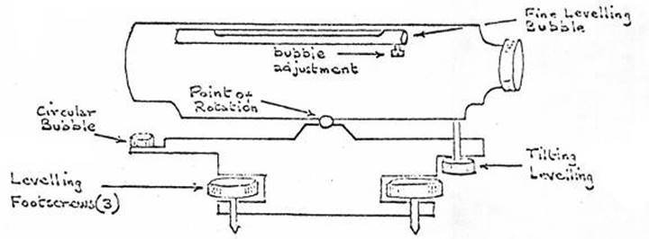
Figure 1.26.1(a)

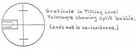
Figure 1.26.1(b)

1.26.2 The Automatic Level

All leading surveying instrument manufacturers now have automatic levels available and at least one theodolite incorporates the system, instead of the alidade bubble, for use when observing vertical angles.

In appearance the automatic level is just like any conventional level; it has the usual three footscrews for levelling with the small circular bubble. However the orthodox bubble attached to the telescope has been abandoned. In its place are three prisms; one system has two of these prisms rigidly connected to the telescope tube with the third hung to swing freely; another system has one rigid prism with two swinging freely. A damper is incorporated to steady the line of sight and the whole unit of prisms and damper is called the "optical stabiliser".

The basic concept of the automatic level is that swinging freely, under the influence of gravity, the stabiliser automatically aligns the line of sight on the wires and in the horizontal plane, i.e., ninety degrees to the plumb line even though the telescope itself is slightly tilted. The range of the stabiliser of a good automatic level is plus or minus twenty minutes (±20¢) and this is well taken care of if the instrument is levelled with the small circular bubble, which however must be kept in adjustment.

It should be noted that most modern automatic levels give an upright image. The automatic level should be carried with the telescope in a vertical position, so that the stabiliser is at rest, when ravelling from job to job. The type of carrying case supplied by the maker usually takes care of this.

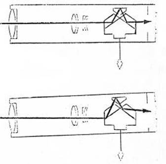
Figure 1.26.2. The Watts “Autoset” stabiliser and principle of operation.

In the “Autoset” level telescope there is the stabiliser consisting of two prisms on a suspended mount.

If the “Autoset” is tilted the stabiliser swings like a pendulum and keeps the horizontal ray on the cross-lines automatically

1.26.3 Level Tripod

The tripod is similar to that used for theodolites, the main difference being the absence of a moveable centring device. The same care should be given to the level tripods as is given to the theodolite tripod or the quality of the observations will suffer; check for loose bolts, screws or ferrules and keep the tripod well varnished.

1.26.4 Staff

Many types of staves are available, however the one most likely to be encountered at present is the "Sopwith" two piece hinged type, or the "Sopwith" three piece telescopic type, both of which are graduated in feet and hundredths.

Figure 1.26.4(b) shows this system of graduating the staff and indicates the method of reading these graduations.

The telescopic staff is easier to carry, however the more rigid two piece hinged type is more accurate since it maintains its length better over a period of time. It also usually has a, circular staff bubble attached, while the telescopic type requires a hand held staff bubble. Needless to say, all staff bubbles must be kept in adjustment.

Foot-metric staves are also available. With these, all readings are taken both in feet and metres, thus providing constant checks and greater accuracy.

All staves should be carefully looked after, kept clean and dry and always returned to their carrying cases when not in use. When carried in the vehicles they should preferably be strapped high up inside the vehicle to prevent damage from digging tools or other heavy sharp equipment, as will occur if the staff is laid on the floor.

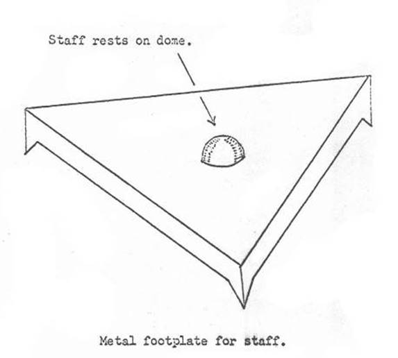
Figure 1.26.4(a)

A steel footplate, upon which to stand the staff at change points, is necessary to ensure a firm base at such points. A suitable type is shown in Figure 1.26.4(a).

Figure 1.26.4(b) Levelling Staff “Sopwith” type.

1.26.5 Testing and adjusting the Surveyors Level

The "Two Peg Test" is used to ascertain any error in either a Tilting or an Automatic level. The test will be described first and the adjustment to each typo of level will be described in general terms. However it is advisable to consult the handbook of the particular brand of instrument in use before adjusting any instrument with which the user is not familiar.

Two Peg Test

(i) Two points A and B are selected 200 feet apart and pegs driven in firmly.

(ii) The level is set up at C, midway between the marks (plus or minus a couple of feet). Carefully take readings to a staff held on A and B in turn. The difference between those is the accurate difference in height regardless of the adjustment of the instrument. This is because the horizontal distances AC and BC are the same; therefore if the line of sight is not horizontal, both staff readings will be an equivalent amount too high or too low. See Figure 1.26.5 (a).

(iii) Move the level to the vicinity of Peg A; set up on an extension of the line AB at minimum focus distance from the peg (about 6 feet). Again carefully take readings on the staff, hold on A and B in turn. If the difference between these two staff readings does not agree with the, difference in height as found when the staff readings were taken from the mid-point, the level needs adjusting. See Figure 1.26.5(b).

Unless the instrument has a large error, it can be considered that the line of sight and the horizontal line as shown at rA in Figure 1.26.5(b) are so close that no different reading on the staff at that point could be made after the bubble was adjusted.

Therefore the reading A of 4.68 - the accurate difference in height of 1.93 would give the point where the horizontal line would cut the staff at B, i.e. 2.75. See Figure 1.26.5(c).

Procedure where the instrumental error is large

If the error is known or thought to be very large, instead of making the second set-up of the instrument at minimum focus from the staff, it should be set up at a known distance on the extension of the line AB. This known distance should be some convenient fraction of the distance AB, for example AB = 200 ft, setup at 20 ft from A, ratio 1:10. Proceed with the test, noting that by similar triangles, a correction to the line of sight will need to be made at both peg A and peg B and that it will be in the ratio 1:10. See figure 1.26.5(d).

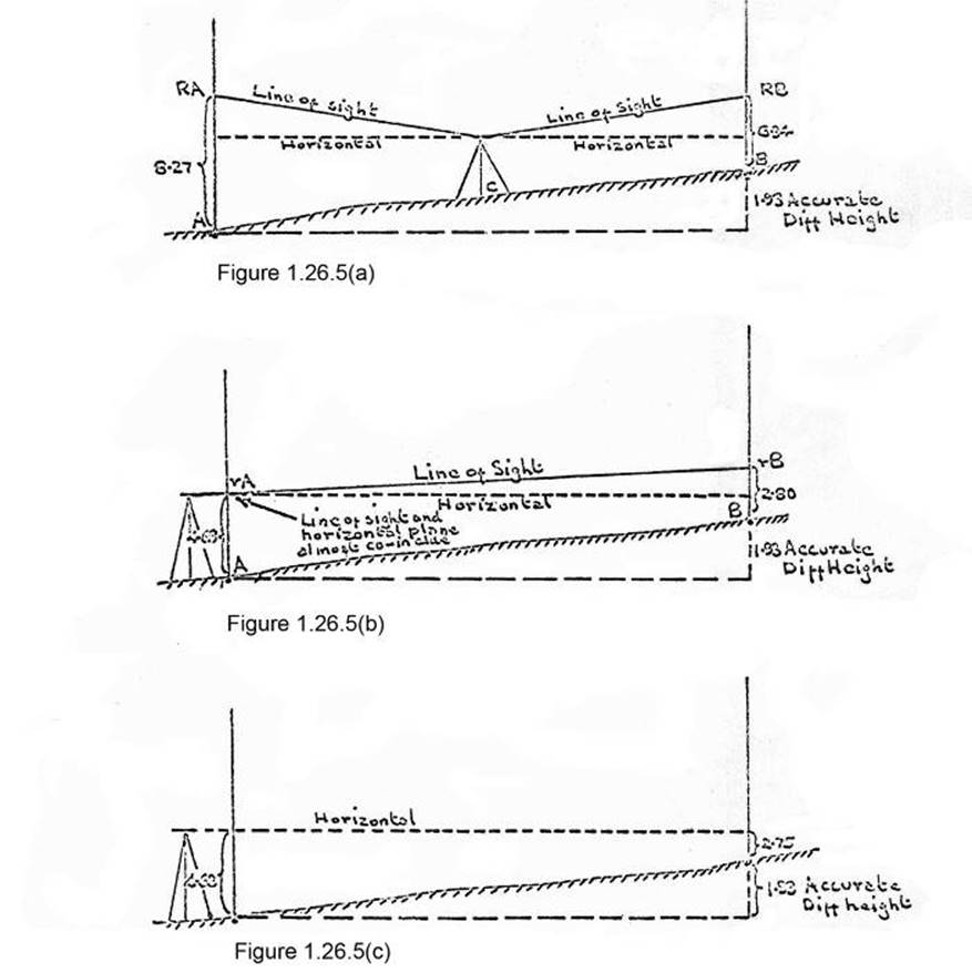
Figure 1.26.5(d). Triangles IHB and IHC are similar;

therefore the error in the line of sight at BH is 1/5 the error at CH.

Adjusting the tilting level after the Two Peg Test

The staff is taken to peg B, and the central crosswire is laid on the staff with the tilting screw at the calculated correct reading, in the case of the example from Figures 1.26.5 (a,b & c) it is 2.75. Naturally this moves the ends of the split bubble apart but the line of sight is now horizontal.

With the bubble adjusting screw, the ends are then brought into coincidence thus the line of sight remains horizontal and the bubble is now in agreement with the horizontal line as defined by the line of sight through the central crosswire of the telescope.

To check the instrument, take a couple of careful readings on the staff which is still at A, bringing the bubble ends into co-incidence with the tilting screw in the normal manner, move the staff to B and repeat. The difference in the readings rA - rB should now agree with the difference height.

Third order levelling specifications state that the vertical collimation error must not exceed ten seconds of arc, which is just on 0.01ft at 200 feet, therefore if agreement is within 0.01ft no further adjustment is necessary. If the difference is greater than 0.01ft repeat the adjustment until this accuracy is achieved.

Adjusting the Automatic Level after the Two Peg Test

The staff is taken to peg B, and the central crosswire is brought onto the staff at the calculated correct reading, in this case 2.75, by means of graticule adjusting screws.

Thus the central crosswire has now been brought into coincidence with the horizontal line of sight as defined by the stabiliser unit and this line will be correct unless the stabiliser has been damaged. To check that the adjustment has been performed correctly proceed exactly as for the check of the adjustment to the tilting level.

1.27 Level Traversing – Hints

1.27.1 The Instrument and type of levelling

The instrument to be used would most likely be the Watts "Autoset", or a similar type of automatic level.

The tasks likely to be encountered will most likely be level traverses with few, if any, intermediate points. In mapping surveys "grids" of levels are rarely required.

1.27.2 Extracts from "Specifications for contract Third Order Levelling

(i) Vertical collimation error of instruments shall not exceed ten seconds of arc (0.01ft at 200 feet). Field tests to be made before work commences each day. Tests to be booked on 1 complete page of the fieldbook immediately preceding that day's level observations. Results are to indicate the error before, and residual error after adjustment, together with distances over which the test were conducted.

(ii) Periodic tests to be made to ensure proper adjustment of the staff bubbles.

(iii) With Automatic Levels:

(a) The circular bubble must be in precise adjustment at all times.

(b) Each time the level is set up to take readings, the dislevelment shall not exceed the tolerance laid down in the manufacturers hand book.

At consecutive bays, level the instrument with the telescope pointing in opposite directions, i.e. at first and third setups the telescope should point towards the backsight, and at second and fourth setups the telescope should point towards the foresight.

When two staves are employed and the staffmen are "leap frogging" this is resolved by always pointing the telescope at the same staff when levelling the instrument.

(d) To ensure the stabiliser is free to oscillate, prior to every reading the telescope is to be turned slightly in one direction then the other.

(iv) Placement of the Staff

(a) Bases to be inspected and cleaned if necessary at every change point. The staff shall always be placed on a steel footplate at each change point, unless change point is a Bench or other station mark, temporary BM, concrete culvert, firmly driven survey peg, etc.

(b) When two staves are being used, there must always an even number of instrument stations between consecutive BM's so that the same staff is placed on the starting mark as a backsight and on the next as a foresight. This eliminates any zero error i.e. the graduations of the two staves.

(v) Length of sights

(a) The length of any sight shall be such as to allow the positive resolution of the staff graduations, and no sight shall exceed three hundred feet, even under conditions of very good visibility. (As a general rule, it is advisable to keep sights to about 200 ft. Also see that the centre of the graticule is kept higher than one foot from the base of the staff to prevent refraction causing errors in rays which are too close to ground level).

(b) As shown in the notes for adjusting the level, back and fore sights should be balanced at the same length to help mitigate any instrumental errors: this is probably best controlled by dragging a standard long rope; when only a short sight can be obtained because of a steep slope, the next sight must be a correspondingly short sight, even though a normal length sight could have been made. Upper and lower stadia readings are always recorded to prove that the sights have been balanced and to measure the overall length of the traverse.

(vi) Accuracy

In general, the forward and back levelings of a section (or, in the case of a loop, the closure on the commencing station) shall not differ by more than ± 0.05 ÖM feet, where M is the distance in miles between the BM's (or the length of the traverse in the case of a loop).

For details of checks for accuracy of all cases that may be met with in third order levelling consult the appropriate specifications, section 5.1.

1.27.3 The Level Field Book : Rise & Fall Method

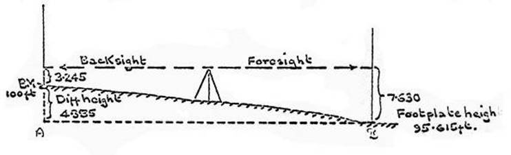
Figure 1.27.3(a)

Figure 1.27.3 shows the procedure when levelling:-

Step 1: The staff is set up on the BM, termed point A in the diagram, height 100 ft.

Step 2: The level is set up about 200 feet from A along the line of advance.

Step 3: The second staff is setup on the steel footplate at change point B, a further 200 feet along the line of advance.

Step 4: A reading is taken on the staff held at A; this is booked as a backsight, and in this example is 3.245 ft. Note that sights of 200 feet or under should be read to the nearest 0.005 ft. Stadia readings to the nearest 0.01ft are also taken.

Step 5: A reading is taken on the staff held at B, this is booked as a foresight, and in this example is, 7.630. If only one staff is available the observer must wait for the staffman to move from A to B before this reading can be taken.

Step 6: As the foresight is larger than the backsight B is lower than A, therefore the difference between the backsight and the foresight is booked as a “fall” in the appropriate column, i.e. 7.630 - 3.245 = a "fall" of 4.385, therefore the height of B is 100 - 4.385 = 95.615 feet.

A suitable field book layout is shown in Figure 1.27.3(b). This is eminently suitable for a level traverse, without intermediate sights and using either a foot or metric staff. In the case where the foot/metric type staff is to be used, the extra columns for metric readings are provided on the right hand side of the field book page. The appropriate lines are "blanked out" to ensure that the first foresight is written one line below the first backsight.

Checking the Reductions

Backsights and Foresights are totalled at the foot of each page, as are the Rise and Fall columns. The difference between the Backsights and Foresights is noted and this should be the same as the difference between the Rise and Fall columns. It should be noted that to apply this method of checking, the first sight on the page of levels must be a backsight and the last sight on the page must be a Foresight, with this entry repeated as a Backsight as the first entry of the next page.

Where a Reduced Level value is available for the commencing BM, Reduced Levels are carried forward in the appropriate column, this gives a further check on the reductions as the difference between the first and last Reduced Levels should be the same as that of the difference between the total Backsights and total Foresights, and the difference between the total Rise and the total Fall.

This book is hardly suitable for use when booking a "grid" of levels with many intermediate sights. In that case it probably would be better to especially rule up a plain fieldbook to suit the task in hand. Where only a few intermediate sights are required the fieldbook described could be used by entering these sights in one of the columns designed for metric readings, providing of course that the foot/metric staff is not being used.

1.27.4 The Level Field Book : Collimation Method

This method which is suitable for certain types of engineering surveys - the booking for a stadia traverse with a theodolite is a variant of the Collimation Method - is unlikely to be met with in mapping surveys; however the following explanation and example is provided.

The method consists of finding the Reduced Level of the line of sight at each station (referred to as the Reduced Level of height of Instrument, or just height of Instrument) and subtracting from this value the reading on the staff at each point to obtain the reduced level at that point:-

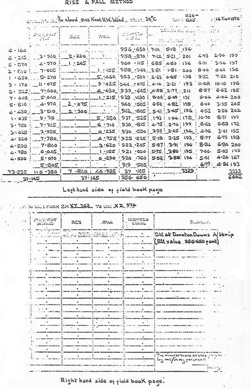
Figure 1.27.3(b)

Step1. This R.L. Line of sight is always found by adding the backsight reading to the R.L. of that station.

Step 2: From this Line of sight, the RL, of the forward station is always found by subtracting the foresight reading on the staff. See Figure 1.27.4(a).

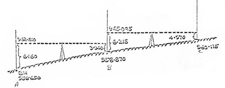
Figure 1.27.4(a)

In the above Figure, RL of A = 956.650 + backsight reading on staff 6.160 = 962.810 which is RL, Line of sight (or height of instrument). Then 962.810 - reading on staff at B, 3.940 = RL of B is 958.870, and so on.

One check only is available, i.e. that on any page the difference between the total backsights and the total foresight should equal the difference between the R.L. of the commencing and final stations on that page, providing of course that the first entry on the page is a backsight and the closing entry a foresight.

Levelling Field Book page.

2 Theodolite – General Description

2.1.0 General Description

The theodolite is an instrument for measuring horizontal and vertical angles. There are numerous types, but they all have the following essentials.

2.1.1 A "lower plate" revolving about a hollow vertical axis, and fitted with a graduated circle. It is also provided with a circle setting screw, so that the circle can be set at any selected point in its rotation.

2.1.2 An "upper plate" which rotates about a vertical axis, fitted into, and concentric with, the axis of the lower plate. To this upper plate are rigidly attached a pair of standards and a levelling bubble. It also carries the horizontal clamp and tangent screw, and the reading device, normally a micrometer.

2.1.3 An "Alidade" which is the name given to the combination which consists of the horizontal axis, telescope and vertical circle together with a levelling bubble. The vertical circle is fitted with a clamp and tangent screw, for use in measuring vertical angles. The "alidade" bubble is fitted with an adjusting screw, either of the ordinary tangent type, or fitted with a lock-nut, to set the zero in its correct position.

2.1.4 Other parts are, levelling screws by which the axes of the plates can be set truly vertical, a traversing head with which the instrument can be moved for a short distance, in any direction, without disturbing the tripod; and a plumbob suspended from the centre of the vertical axes, with which the instrument can be set up, vertically, above a point on the ground.

2.1.5 For a theodolite to be in perfect adjustment, the following requirements must be fulfilled:-

(a) The horizontal axis must be truly perpendicular to the vertical axis.

(b) The line of sight, as defined by the cross hairs in the telescope, must be truly perpendicular to the horizontal axis.

(c) The centre of rotation, of the upper plate, must coincide, with great precision, with the centre of the graduations of the circle, on the lower plate.

(d) At least one levelling bubble must have its axis truly perpendicular to the vertical axis.

(e) The alidade must be so adjusted that, when the vertical axis is vertical, the reading on the vertical circle correctly indicates the inclination of the line of sight.

2.1.6 When these conditions are fulfilled, if the instrument is "Levelled" (i.e., if the, levelling screws are adjusted until the bubble remains central, for a complete revolution, about the vertical axis) it will be possible correctly to read horizontal and vertical angles.

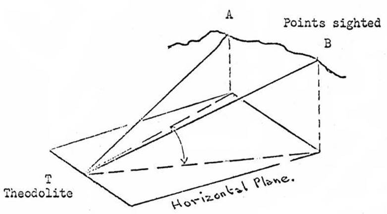
Figure 2.1.7.

2.1.7 It must be realized that when the instrument is in adjustment, the line of sight traces out a vertical plane, at right angles, to the horizontal axis, as the telescope is elevated, or depressed.

If the theodolite is set up at "T" (Figure 2.1.7.) and the telescope directed, in turn, first to "A" and then to "B", the angle read is the angle between the vertical planes passing through TA and TB. That is to say, if perpendiculars are dropped from A and B to the horizontal plane containing T, the angle read is that subtended by the feet of these perpendiculars, and not by the points A and B, themselves, unless those points happen to be on that horizontal plane.

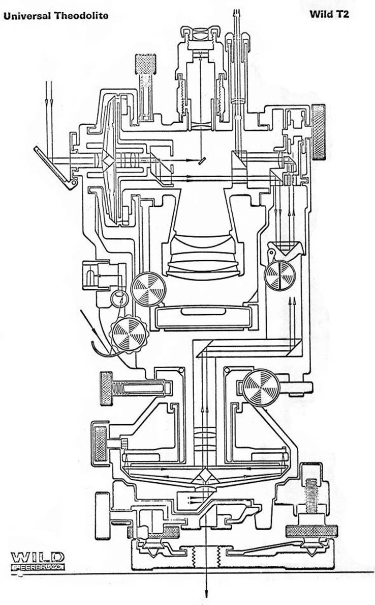
3 Theodolite – WILD T2 - its use in all types of observation

3.1. General preparation.

While not the official Wild T2 manual this version provides very similar information.

3.1.1 Care and adjustment of the instrument and tripod

At the end of each field season, the theodolite will normally be completely overhauled by the maker, or agent, and should be issued in tip top condition for the season’s work. Only minor adjustments are to be made by the party leader or observer, in the field.

Before leaving for the field the instrument should be checked to see that no fault has been overlooked in the laboratory by the maker or agent. Mainly, these will be:-

(a) All lenses not cleaned.

(b) Telescope lighting inadequate.

(d) Horizontal collimation is within a few seconds.

Any of the above faults should be rectified immediately they cannot be done under field conditions.

3.1.2 The minor adjustments which can be done are :

(a) Adjustment of tension of slow motion and footscrews with the capstan bar provided.

(b) Centralising the plate bubble, if badly off centre. This is done by levelling the instrument inside a screen (or in the shade), then bringing the plate bubble close to the central position, with a capstan bar. This is not a precise adjustment as the bubble will almost certainly move off a little, during the season.

(c) Adjustment of vertical collimation : This is done by reading a FL and FR vertical angle to a prominent point. If these 2 angles agree within a few seconds, no adjustment is necessary. If not, mean the FL and FR angles to get the true vertical angle to the prominent point. Then proceed as follows :

(i) Lay on prominent point, clamping lightly both horizontal and vertical circles.

(ii) With alidade bubble setting screw, set the vertical circle to read the true vertical angle. While doing so, notice that the bubble ends, as viewed through the prism, will move apart.

(iii) Using the screw provided for adjusting the Alidade bubble, the ends of this bubble are brought into co-incidence, as viewed through the prism, and the adjusting screw is locked.

The vertical circle has now had the collimation error eliminated. It is advisable to again read the FL and FR vertical angles to check that the adjustment has been successful.

(d) The lighting set should be checked, by the observer prior to the commencement of the season. See all connections are clean and firmly soldered, and the rheostat free from rust. If it is not allowed to get wet, the lighting set should give no trouble during the season. Power supply is three, 1.5 volt dry cells coupled in series, and packed in a plywood box. The rheostat should be turned well down while the dry cells are new.

(e) Maintenance. Keep the theodolite clean, and all parts free from dust, at all times. Use a camel hairbrush and lens tissues, also cover the instrument with a plastic bag, when set up and not in use.

3.1.3 Tripod

This should be re-varnished at the end of each field season, and left stored with all bolts slackened, in case humidity expands the timber. Before again using the tripod, check that all bolts are tight, and that there is no movement at any point where the timber fits into any metal socket, either at the head or foot, of the tripod. This should be done each day the instrument is used, particularly if the weather is getting drier and hotter. The tripod should be wrapped in hessian or canvas for vehicle transport.

3.2.1 Setting up the instrument

The tripod should be set over the station or eccentric mark so that the height is just right for the observer; no straining because it is too high, and no excessive stooping because it is too low. However; it is better a little low, than too high.

When the instrument is too high, there is a tendency to drag it off level; or to fail to get rid of parallax, owing to the eye not being directly behind the telescope. If azimuths are to be observed as well, the tripod must be oriented so that the instrument can be set up with two footscrews along a north south line.

Once the tripod has been positioned, pegs should be driven if at all possible. 450mm x 75mm square wooden pegs on firm soil, 1 metre x 75mm square for sandhills, or 300mm to 450mm steel pegs on rocky hills. If unable to drive in all pegs, put in as many as possible. Set feet in plaster of paris (use plenty) where pegs cannot be driven. See that when driving pegs, the tripod has not become displaced from its original position, tilting the head badly from the horizontal, and displacing the centre of the tripod from a position vertically over the mark, thus making it impossible to plumb the instrument accurately over the mark, without overhanging the tripod head.

Spend some time in clearing the observing platform of rocks, either loose or partly buried; stamp near each leg, and check for any slight movement of the instrument or tripod. Remember that a partly buried rock, well clear of the tripod, may touch other buried rocks, which in turn, do touch the tripod feet.

3.2.2 Observing screens

This is set up to give plenty of room to move around the instrument; see that the screen poles are not on line to the distant stations; and star, if azimuth is to be observed.

3.2.3 Levelling the Wild T2 theodolite for second order observations

This is done in two stages:-

(a) Fairly accurately, with the plate bubble.

(b) Final accurate levelling with the alidade (split) bubble.

Stage (a):-

Firstly, bring the plate bubble along the line of two foot-screws, and note the position of one end of the bubble, say the vertical circle end. See Figure 3.2.3(a) Turn through 180°, note the position of the same end of the bubble. (Figure 3.2.3(b)) Correct by half the difference of these positions, turn through 180°, until the bubble is level over the two foot-screws. Then turn through 90°, where the bubble will be in line with the remaining footscrew; Figure 3.2.3(c) shows this position. Use the same method to level the instrument along this line, with the single footscrew, this time.

Stage (b):-

Now bring the alidade bubble along the line of two footscrews, bring the bubble ends, as seen through the prism, into coincidence, and turn the theodolite through 180°. Note the amount of error. Take half out with footscrews, and half with the alidade screw. Turn instrument through 180°, and repeat until level along the line of these two footscrews. Now turn through 90°, so bubble is aligned over the remaining footscrew, bring bubble into coincidence, turn through 180°, note amount of error, take half out with remaining footscrew and half with alidade screw. Turn through 180°, and repeat until level along the line of this footscrew. The instrument is now completely level. When shielded properly from the sun, and strong winds, the Wild T2 will hold the level for long periods. It should be remembered to position the footscrews approximately centrally, before commencing levelling.

3.3.1 Horizontal and Vertical scales

While it is not difficult to focus the telescope and scales, great care must be taken, or the observations will be below standard. Remember, as all observers eyes are different, no one else can help by checking your focus.

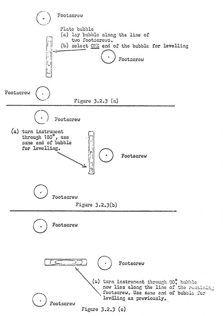
The telescope:‑

(a) Elevate the telescope to the sky, and bring the crosshairs to the clearest and sharpest focus obtainable, by turning the ocular focusing lens.

(b) Sight distant station through the telescope, and focus until the distant station is also clear and sharp.

Move the eye around, when both crosshairs and the distant station are in focus, there will be no relative movement (parallax) between them. Once it is dark, and the light is turned on, in the telescope, invariably, both the distant station, and cross-hairs will need re-focusing.

The scales:-

Always use the lighting set to illuminate the scales (except for reference mark work, around the station.) Carefully focus the scales until the figures are sharp and clear. There may be a slight difference in focus between the horizontal and vertical scales but this rarely matters.

3.3.2 Types of horizontal and vertical scales

The following is an explanation of the Wild T2 theodolite scales these being the instrument mostly in use. However, the observer need only to master the technique of reading the Wild system, to easily change to whichever Wild theodolite is at hand.

3.3.3 Horizontal Circle

This is graduated to 20 minutes, and the 10 minute is found by interpolation. The micrometer drum is graduated to 1 second, with a run of 10 minutes. Looking into the scale telescope, two windows are seen. In the top window, by means of prisms, two diametrically opposite sections of the horizontal circle are seen, one the correct way up, and the other upside down. An index line is shown in the centre of the scale. In the bottom window, a section of the minute and second scale, with index line, is seen.

3.3.4 Reading the horizontal circle

When the micrometer drum is turned, the minutes and seconds will move past their index line, and the opposite sections of the horizontal circle, will move so that the graduations appear to approach one another movement of the micrometer drum is continued until the equivalent graduations of the horizontal circle are brought into coincidence. Now the index line, in the upper window, will either coincide with a graduation mark, or will come half-way between two. In the former case, the degrees and minutes are read direct, using the 20 minute mark which coincides with the index mark; in the latter case, interpolate to the ten minute lying between the two 20 minute marks. The reading on the micrometer scale gives the number of minutes and seconds to be added to the degrees, and tens of minutes, read on the main scale. Figure 3.3.4 shows an example, and mentions an alternative method of ascertaining the value of the divisions.

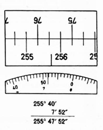
Figure 3.3.4. Horizontal circle

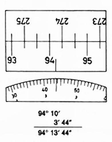
Figure 3.3.5. Vertical circle reading on one face only.

Figure 3.3.4. shows the image in the reading microscope eyepiece after coincidence. In the upper window, the index line shows the approximate value will be close to 256° and the first upright figure left of the index line, shows a reading of 255°. Now count the intervals from 255° to the diametrically opposite 75° mark. There are 4 intervals, that is, four tens of minutes, or 40'. A reading of 255° 40' is thus obtained from the upper image. In the lower image of the seconds drum scale, we read 7 minutes and 51.8 seconds. Thus shown on the drum, the complete reading is 255° 47' 52", the nearest second always being recorded.

3.3.5 Vertical circle

The vertical circle on the Wild T2 is graduated similarly to the horizontal circle. However, it should be noted that on FL it reads ZENITH DISTANCE, and on FR, 180° plus the zenith distance.

As the altitude is normally the vertical angle required (however the Sun azimuth proforma uses the zenith distance) it will be necessary to make the following calculations:-

Face left :

If the observed angle is less than 90°, take it from 90°, and the answer is a FL angle of Elevation.

If the observed angle is more than 90°, take 90° from it, and the answer is a FL angle of Depression.

Face right :

If the observed angle is more than 270°, take 270° from it, and the answer is a FR angle of Elevation.

If the observed angle is less than 270°, take it from 270°, and the answer is a FR angle of Depression.

The mean of the FL and FR angles gives the altitude free from collimation.

3.3.6 Reading the Vertical Circle

The graduations are read in exactly the same manner as with the horizontal circle, with the exception that immediately before the graduations are brought into co-incidence, the two ends of the alidade bubble, as viewed through the prism, must be brought into coincidence. The horizontal cross-hair has been set exactly on the aiming point, and the alidade bubble ends brought into coincidence with the tangent screw. Then the diametrically opposite graduations of the vertical circle are brought into coincidence, by turning the micrometer drum.

The reading from the upper window is : 94° 10¢

and from the lower window : 03¢ 43.8²

Thus the full reading (always to nearest second) : 94° 13¢ 44"

3.4.1 Observing

The following method of observing horizontal angles (most of which also applies to observing azimuths) has been designed so that all movement becomes automatic, and the hands always go to the right control on the instrument, whether in daylight or darkness. Also, to eliminate errors, which could result from friction, or any slight wear of the instrument. Once the technique is mastered, the observer should work quickly, and smoothly, acquire a very light touch on the instrument, move quickly, but carefully, around the instrument. It should be turned with two hands, one lightly holding each standard, not by the end of the telescope.

Targets normally will be either opaque beacons, helio's, lights either in daylight or immediately after dark.

Observations will be made in the last couple of hours of daylight or immediately after dark. In theodolite and tellurometer traversing generally only two distant stations will be observed.

3.4.2 Double pointing system

Most time is consumed in locating each distant station, and the greatest source of error in observing, is pointing at these targets, therefore, once the target is located, much greater accuracy is obtained if two distinctly different pointings are made, the micrometer drum being read at each pointing. This method is known as double pointing.

Before commencing observing, see that both horizontal and vertical slow motion screws are centrally positioned, to ensure an equal amount of movement, in both directions.

The rear station of the direction of advance of the traverse will normally be the reference object (R.O.), so that any traverse angle shown in the field book; will be the clockwise angle from the rear to forward station. On face left, bring this target between the double wires, set about 30" on the micrometer drum, and with the circle setting knob, set the circle to 00° 00'.

The instrument is now ready to commence observations, proceed as follows:-

(a) Face left, swing left through 360° until the R.O. is close to the cross wires in the telescope, clamp the instrument, and bring the target centrally within the double wires, (fairly close to the horizontal wire) using the horizontal slow motion screw and making the last movement of this screw, a "screwing in” motion against the spring. Bring the scales into coincidence with the micrometer drum, the last movement of which should also be "screwing in". Read the angle, move the cross wires clear of the target with the slow motion screw, and again centralize the target within the double wires, once again making the last movement of the screw, as previously. (This movement of "screwing in" the slow motion screw is most importnat to keep tension against the spring. Remember also that when the instrument is on face right, the screw is on the opposite side of the theodolite to the observer, therefore, great care must be taken by the observer to ensure he still uses the "screwing in" motion on this face). Bring the scales into coincidence and read the angle. If the pointings are over 3" apart, discard both, and take two more. If still wide apart, the focus is probably incorrect, on either telescope or scale, or both. If the focus of the instrument is satisfactory, conditions must still be unsatisfactory for observing.

(b) Unclamp the theodolite, swing left until the distant station is close to the vertical cross wires (and about a similar distance from the horizontal cross wire, as was the R.O.). Repeat exactly as in (a). If the instrument is swung too far past the station to lay on the target with the slow motion screw, continue the swing, in the same direction, through 360°.

(c) Unclamp the theodolite, change to face right, swing right until the same station is close to the cross wires, clamp, and repeat as in (a).

(d) Unclamp the theodolite, swing right, until the R.O. is close to the cross wires, and repeat as in (a). That completes the observations on this scale setting.

(e) Set micrometer drum to 03¢ 50", set scale to required setting with circle setting knob (in this case 240° 00'). Swing right through 360° and bring target centrally between the double wires, as previously explained. Continue observing in this manner, until 6 arcs, which comprise one set, are completed.

3.4.3 Scale settings

		1st Set			3rd Set				5th Set
FL	000°	00'	30"	15°	001			20°	00'	30"
FR	180°	00'	30"	195°	00'	30"		200°	00'	30"
FR	240°	03'	50"	255°	03'	50"		260°	03'	50"
FL	60°	03'	50"	75°	03'	50"		80°	03'	50"
FL	120°	07'	10"	135°	07'	10"		140°	07'	10"
FR	300°	07'	10"	315°	07'	10"		320°	07'	10"

		2nd Set			4th Set				6th Set
FR	210°	02'	10"	225°	02'	10"		230°	02'	10"
FL	30°	02	10"	45°	02'	10"		50°	02	10"
FL	90°	05'	30"	105°	05'	30"		110°	05'	30"
FR	270°	05¢	30"	285°	0.5'	30"		290°	05¢	30"
FR	330°	08¢	50"	347°	09'	55"	random	350°	08¢	50"
FL	150°	08'	50"	167°	09'	55"	arcs	170°	08'	50"

Settings are slightly approximate.

Naturally, on return to the R.O., collimation will give some variation to the original settings.

Each of the above sets is meaned, and normally, at least 4 to 6 sets are observed.

Usually, the range in each set is about 5", with an odd arc to 7" or 8"; however, if conditions are difficult, this range may not be achieved. Once the observer is experienced, and carefully and conscientiously observes the targets, and scales, as he sees them, the spread in the arcs is really a measure of the observing conditions. Thus results below standard, by an experienced observer, would indicate the need to re-observe that station under better observing conditions.

3.4.4 Check or random arcs

From a random, initial setting on the R.O. in any one of the sets, two arcs are read just as carefully, in the normal manner, to the distant station. This is to ensure that the degrees and minutes, have not been read consistently wrong. The usual care in reading those arcs, is required so that they can be used in the set. There is such a short period of good visibility each evening that full advantage must be taken of it.

3.4.5 Booking horizontal angles

The booker will record the name and/or number of each station observed, also the type of target observed. The observer will call out the degrees and minutes, a slight pause during which the booker calls back the degrees and minutes. The observer, who has read the micrometer drum, for the first pointing, during the pause, calls out the "seconds" reading; points again, and calls out the "seconds" reading, once again. The booker calls back these readings, as he records them.

All calling out should be sharp and business-like.

The booker should mean the two seconds readings, and subtract the mean reading on the R.O. from the mean reading on the distant station, as the observations are being taken, meaning these answers at the bottom of the page, when the set is completed. See example Figure 3.4.5(a).

At the conclusion of the night's observations, the observer will check all reductions and the means of the sets. Both booker and observer will sign each page. The observer should cover the previous answer with scribbling paper, while he completes his checking, to get a completely independent answer.

3.4.6 Vertical Angles

These will be truly simultaneous, and should be read between 1400 hours and 1600 hours LMT (Local Mean Time), when the air is most evenly heated. However, if lines are less than 16 Km (10 miles) in length, they may be observed between 1000 & 1700 hours, but still must be observed simultaneously. Lines less than 3km (2 miles) in length may be read non-simultaneously.

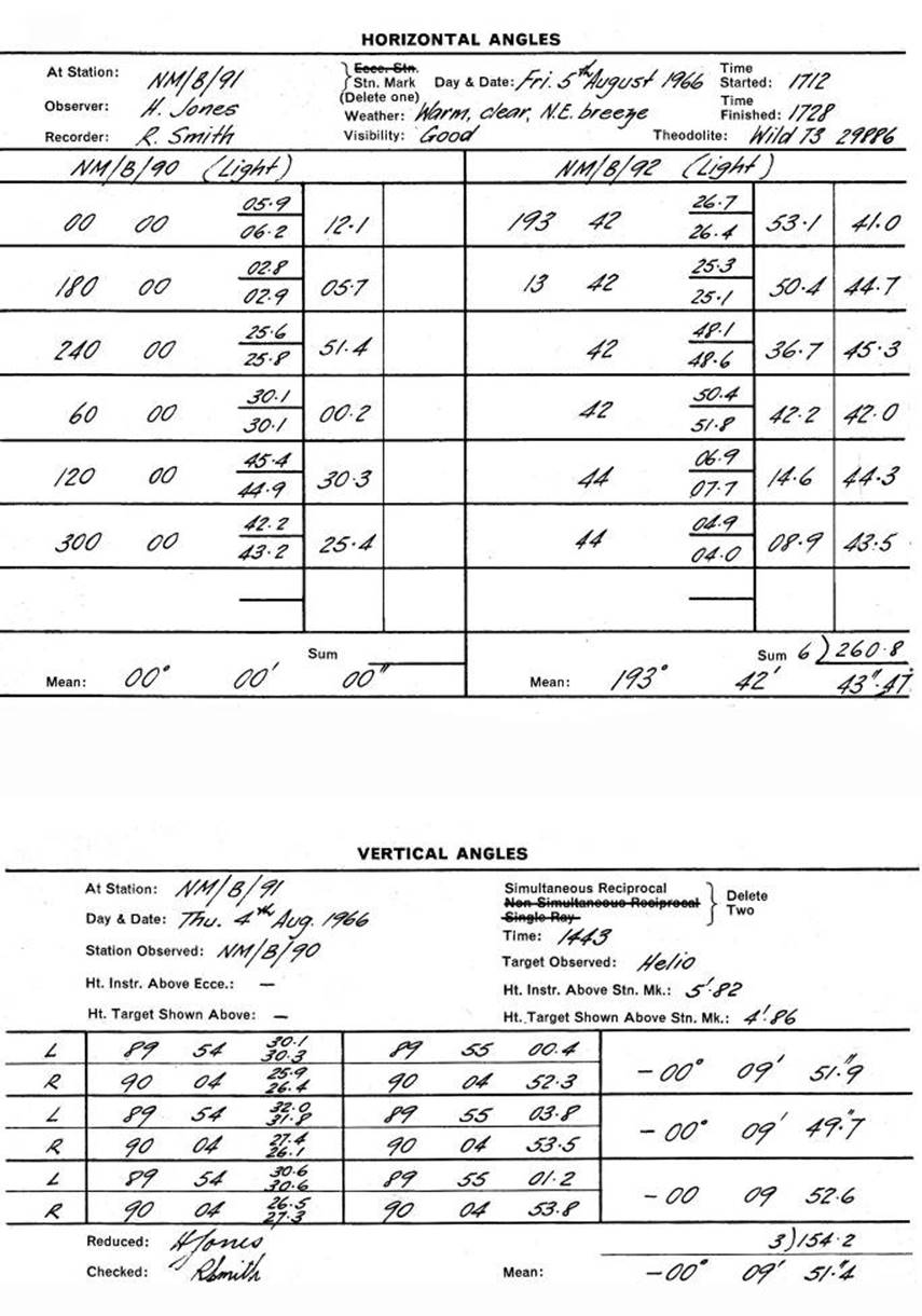
Figure 3.4.5(a) – Booking Horizontal Angles and Figure 3.4.10(a) - Booking Vertical Angles.

3.4.7 Probably the best type of target over the average length of line is a hello, and for shorter lines, the daylight (Flamethrower) lamp. The top of the vanes makes a fair target on lines up to 32km (20 miles) in length, if the lines have a good drop away at each end. Heights of targets above a station mark (or below, in rare cases) must always be recorded.

3.4.8 Screens should always be used for vertical angles; normally at the time of observation the sun will be beating strongly on both the instrument and tripod, unless they are shielded. If conditions are not too windy, and the time is short, a makeshift shelter which completely shades the instrument and tripod will suffice; i.e. the vehicle and part of the observing screen, or swag cover, etc.

3.4.9 Observing technique

A similar system of double pointing to that used for observing horizontal angles, is used for observing vertical angles. To keep in line with this system, it is essential that the alidade bubble ends are brought into coincidence just prior to each reading of the micrometer drum, even though the ends appear to still be in coincidence from the previous reading. This helps to even out erroneous readings arising from "flat" spots in the grinding of the level vial.

Observing procedure:-

(a) Face left, intersect the target with the horizontal cross wire close to the central vertical wire, making the last movement of the slow motion screw against the spring, i.e. "screwing in".

(b) Bring the alidade bubble ends into coincidence, in the same manner, read the graduations on the scale, Move the alidade bubble slightly off, move horizontal cross wire slightly off, then intersect the target once again exactly as before, again bring the bubble ends into coincidence, and again read the graduations on the scale.

(c) Change to Face right, and repeat as above. The difference between the readings obtained on these faces, is the vertical angle, and 3 such angles make up a set. To be sure of best results, the observer must change face after each pair of double pointings.

3.4.10 Booking vertical angles

On face left, after pointing on distant station, and levelling alidade bubble, the observer will call out the degrees and minutes, a slight pause during which the booker calls back the degrees and minutes. The observer, who has read the micrometer drum for the first pointing, during the pause, calls the "seconds" reading, points, and levels the alidade bubble again, then calls out the “second” once more. The booker calls back the readings as he records them, and should mean the seconds readings, bringing the Face Left angle forward, into the next column to the right, in the field book. The observer changes to Face Right, and both observer and booker, repeat the above. The booker means the FL and FR vertical angles, and brings the resultant answer forward to the last column on the right, in the field book. When three such angles have been obtained, the set is complete, and the mean is brought down to the bottom of the page. Measure and record, heights of instrument and targets above station mark. See Figure 3.4.10(a) for an example.

The observer will check the reductions, and both will sign each page. The booker should check that there is no gross error, in the degrees and minutes, while the observation is in progress, by noting the approximate total of the readings on both faces. This should be about 360°, unless the instrument is badly out of adjustment.

3.5 Measuring and Recording Reference Marks, Eccentric Stations, and Recovery Marks

(This section is to be read in conjunction with 1. Chaining and 7. Station Marking)

The normal method adopted for measuring reference marks, has been to set a theodolite over the station mark (if accessible) or if not, an eccentric mark, and measure all distances by vertical angle and slope distances. Horizontal angles related to a distant station, and the station mark where applicable) are also observed. As marks are usually within 4 to 10 metres, the tops of hills rough with large boulders, and generally windy conditions prevail, the above method has been found to be more accurate than horizontal measuring with tape and plumbobs. If time permits, set up over a second mark, so that all distances can be checked by calculation.

If time is short, measure tie distances, horizontally with tape and plumbobs, and check slope distances by direct horizontal measurement. There should always be three reference marks.

It is impossible to cover all problems which will be encountered at the various types of set ups, however the following three will cover most cases.

3.5.1 Where the station mark is accessible

Set the theodolite over the station mark. Lay on a distant station as RO, and set 00°00'05" approximately on the horizontal scale. Read horizontal and vertical angles to each mark on FL. Change to FR and do the same, but this time, measure slope distances, while laid on each RM. Measure height of instrument above station mark.

If plenty of time, set theodolite over one of the RMs and with 00°00' 05" on the scale, lay on the station mark, read horizontal and vertical angles to the station mark and RMs on FL; change face, read angles and measure slope distances and height of instrument. See figure 3.5.1(a).

If time is short, measure tie distances horizontally with tape and plumbobs. See figure 3.5.1(b).

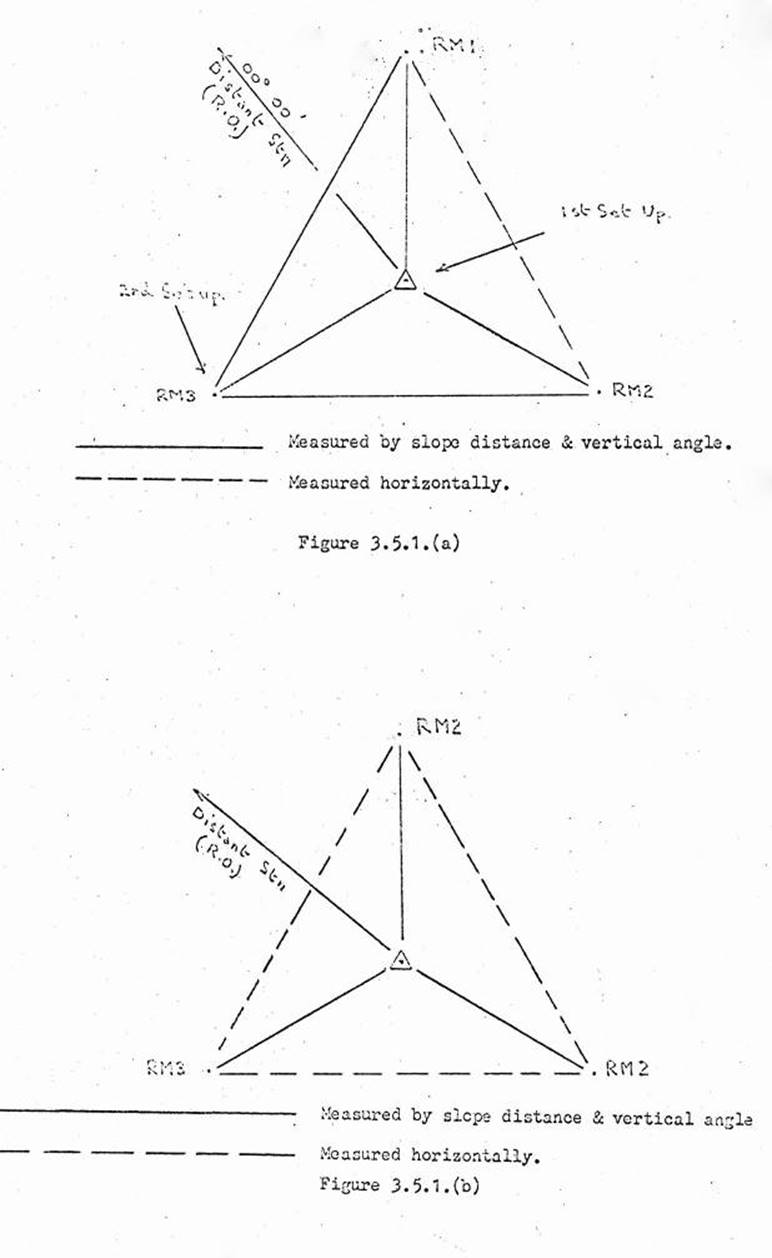
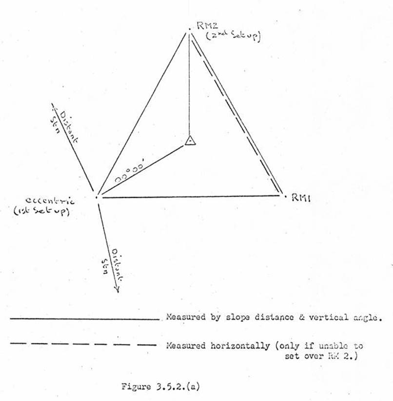
3.5.2 Where the station mark is inaccessible

This will normally be where a large cairn with pole and vanes, covers the station mark. If this is a new station, the distance, eccentric mark to station mark, will have been measured by the beaconing party, as will also the horizontal angles to the two RMs. This data must be with the observer who will lay on the centre pin on top of the beacon with 00°00'05" set on the horizontal scale. Read horizontal and vertical angles to the station and reference marks. Also measure height of instrument, slope distances, cut in at least one of the distant stations. The observer will check against the data supplied, for gross error in the original work of the beaconing party wherever possible, also set up over an RM, and read horizontal and vertical angles to the station mark, eccentric mark and the other RM, on both faces of course. Measure the remaining distance horizontally. See figure 3.5.2(a).

3.5.3 Where there is a distant recovery mark

(This section should be read in conjunction with 7.2.3)

This type of mark will only be placed where the station mark is likely to be lost, either permanently or temporarily i.e. on a sandridge which may erode, swampy & ground or tidal flats. When the above conditions occur, a substantial recovery mark (or marks) will be placed on the nearest firm ground.

Set up the theodolite over the station mark, lay on a distant RO, and set 00°00'05" approximately on the horizontal scale. Read horizontal and vertical angles to the recovery mark, and the two base terminals.

Set over the recovery marks and the two base terminals, in turn, reading all horizontal and vertical angles, thus closing both triangles. Be sure to measure all the heights of instruments, and heights of targets. These observations must be done in good visibility. Targets must be carefully plumbed, and very small; i.e. tripods with plumbobs (laying on plumbob string near hook). If care is taken, the triangles will close within about 10" to 20". Each, almost exact, 100 metre base line is to be measured twice (with an invar tape, if possible) the tape being laid on the ground, temperature taken and a pull of 6.800 kg (about 15lb) applied. This must be done in the very early morning, when the temperature is cool. If a 50 metre band is used, pull will need only to be about 4.600kg (10lb).

Figure 3.5.3 shows a typical Recovery Mark and base line. In 7.2.3 the preparation of the base line, and the Recovery Mark, are described.

All angles are read, so that distance, Station Mark to Recovery Mark, can be calculated from each triangle.

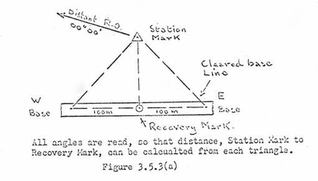
3.5.4 Reference Mark measuring

Figure 3.5.4(a) gives an example of measuring from 2 different set ups. The station mark is covered by a large cairn. Pages, appropriately ruled, are provided in the Traverse, Trig., and Azimuth field books for this purpose.

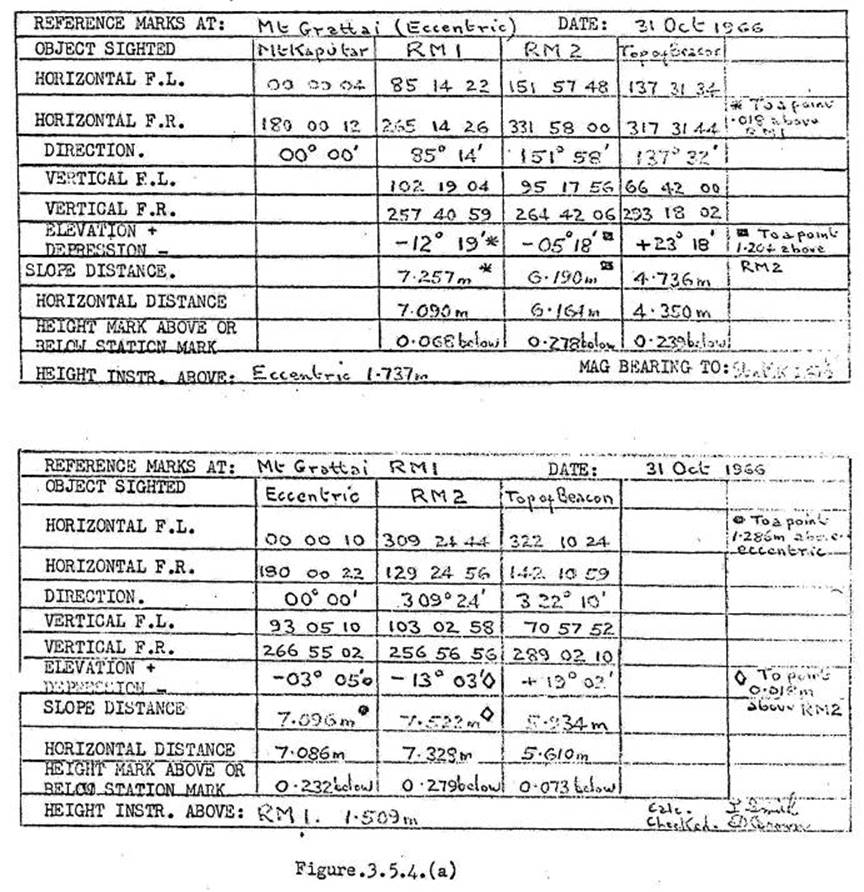
3.5.5 Computation of Reference Marks

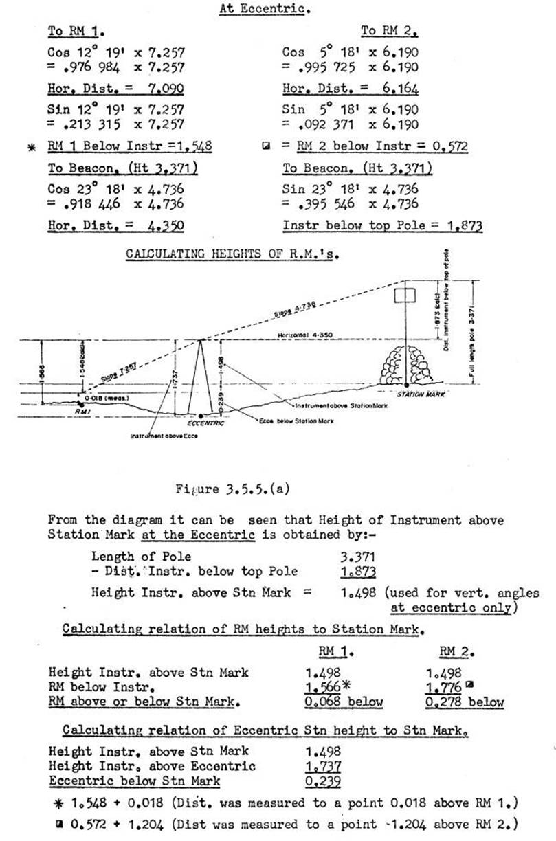
Where the theodolite has been set over two reference marks, all distances can be checked by simple calculation using the formula:-

a/Sin A = b/Sin B = c/Sin C

See Figures 3.5.5(c) and 3.5.5(d) for examples.

Where only two sides, and the included angle are known, the remaining sides and angles can be calculated, as shown on the proforma Figure 3.5.5(e). Where Measurements have been made twice, they should normally agree within 3 to 4mm. If over 6mm measure again. Calculated checks should also have about the same agreement, if the triangles formed, are reasonably well shaped.

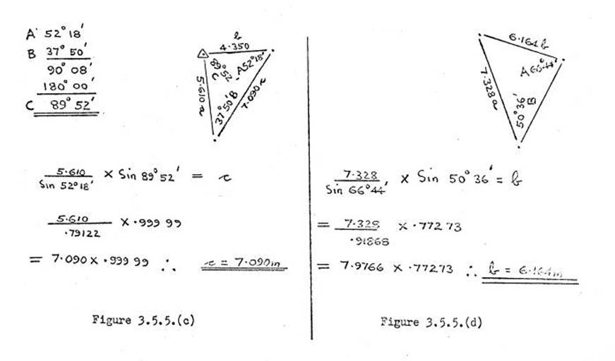
3.6 Eccentric Corrections

3.6.1 Formula

Eccentric corrections, which many find difficult to understand, are really quite simple, once the principle is grasped.

The Sine formula is used:—

a/Sin A = b/Sin B = c/Sin C

The distance, Eccentric Station to Station Mark, is required, also the angle (at the eccentric) between the Station Mark and the Distant Station(s).

The distance to each distant station is required. This does not have to be exact; thus distance, eccentric to eccentric as measured by the tellurometer is quite accurate enough.

3.6.2 Computation

In Figure 3.6.2(a), the bearing, or direction, we have is from the eccentric to the distant station, and we need the correction to apply to it, to get the bearing from the station mark to the distant station. The broken line, from the station mark has been drawn parallel with the line, eccentric to distant station therefore, it is on the same bearing.

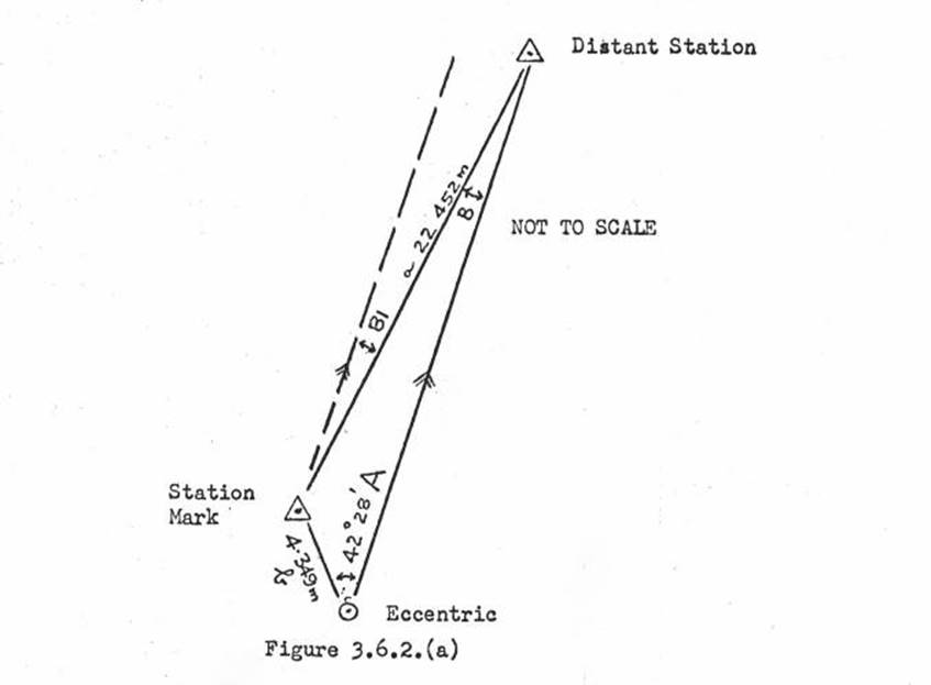
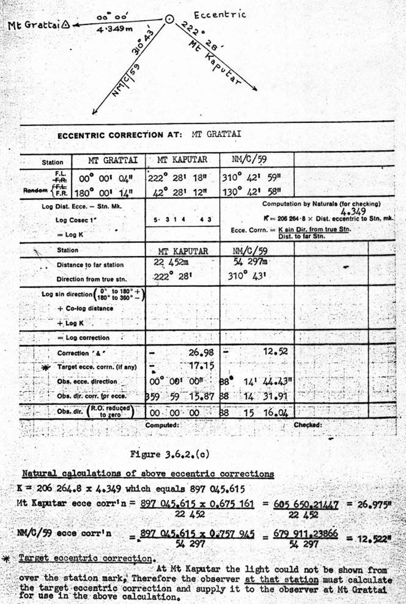
The eccentric correction is the angle B1, and, as the bearing is greater, the sign is +.

B1 is the same value as B, therefore the calculation is:-

a 22 452 = b 4.349

Sin A 42º 28’ Sin B

Sin B = Sin 42º 28’ x 4.349 / 22 452

Log 4.349 0.638 39

Log Sin 42º 28’ 9.829 41

Sum 0.467 80

Log 22 452 - 4.351 26

Log Sin Ecce C'n 6.116 54 (between 26 & 27 seconds)

+ 5.314 43 (Log Cosec 1")(*)

Log Ecce C’n 1.430 97 (in seconds)

Ecce C'n + 26.98"

(*) This is applied so that the angle can be looked up as a direct logarithm (rule for small angles; Chambers Tables).

The above formula is used in the proforma in the field book. However, to avoid subtractions, in the calculation, the Co-log of the distance, Station Mark to Distant Station, is used; and the Cosec 1" is added to the distance between Eccentric and the Station Mark, to give Log "K", and save 1 line in the main addition.

It should be noted, where the angle at the eccentric station, between the Station Mark and the Distant Station is under 180°, the correction is plus, and where the angle is more than 180°, the correction is minus. If in doubt, draw a thumb-nail sketch. See Figure 3.6.2(b) for an example of an eccentric correction, worked out on a proforma.

3.6.3 Small corrections to observations where target at the Distant Station is slightly off line.

The following plotted method is normally used where targets are eccentric by small amounts only, up to 1 metre. If care is taken it is quite accurate. It is also a valuable check for gross error in ordinary eccentric corrections:-

(a) Plot station "A" (Station where target is eccentric) with ray to station "B" (Station where observations are being made to "A"). Use magnetic bearing for plotting this ray which is not to any scale. Note distance to nearest Kilometre against this ray.

(b) At a suitable scale, plot eccentric target by magnetic bearing and distance, which should be in mm.

(d) The eccentric correction will be the amount this distance subtends at the distance between stations. Use the close approximation that 1 second of arc = 5mm per Kilometre.

(e) The 2 examples below show the two types of plot required to cover all situations.

(f) It is easy to decide, by inspection of the plot, whether the direction observed is too great or too small, and thus give the corrections its appropriate sign.

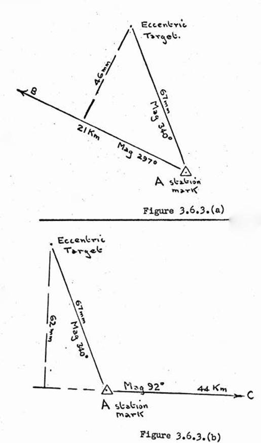
Refer Figure 3.6.3(a) : Target is eccentric by 67mm on a Mag. Bearing of 340°. This gives a distance off line of 46mm from plot.

Calculation:- 5mm x 21km gives 105mm per sec at 21km. Correction is 46mm, which means correction in seconds will be about 0.5" or 105/46 = 0.44".

Looking in from B it is seen that the bearing observed is too small, therefore correction is plus.

Refer Figure 3.6.3(b) : Same target is sighted from C. This gives a distance off line of 62mm from plot. Note that ray A to C has to be extended to measure right angle distance which target is off line.

Calculation:- 5mm x 44Km gives 220mm per sec at 44 Km. Correction is 62mm, which means the correction in seconds will be about 0.3² or 220/62 = 0.28"

Looking in from C, it is seen that the bearing observed, is too large, therefore the correction is minus.

3.6.4 To ascertain amount of lean on a pole, the base of which is a cairn

(a) Mark a line around the pole, 1 metre, or some other suitable distance, from the top.

(b) Stand about 7 metres from the cairn, and at right angles to a face of the pole, point "A" in the diagram 3.6.4(a).

(c) With plumbob, sight edge of pole at "X", and mark x vertically above, on the top edge of the pole. If greater accuracy is required, use the theodolite, instead of the plumbob. Measure distance from corner of pole C to x. This is the amount of lean over 1 metre. If this was 20mm, the lean over the full length of the normal 3.380 metre pole would be:- 20 x (3.38 /1) = 66mm.

(d) Mark this distance along the top edge of the pole, from corner C and call it point “a”.

(e) From “a” draw a line across the top of the pole, parallel with the edge.

(f) Move around 90° to point B and repeat all in (b), except that the last point to be marked will be "b".

(g) The point where lines "a" and "b" cross, at "c", is the point where the corner of the pole C would be, if the pole had no lean. Measure distance "c" to C, and take Mag. Bearing from "c" to C.

Record that pole leans on a bearing of ...° for a distance of ...mm.

(h) From the centre of the leaning pole at D, mark true centre of pole at "d", using above bearing and distance. Take all measurements angles to RM's, and distant stations from point "d".

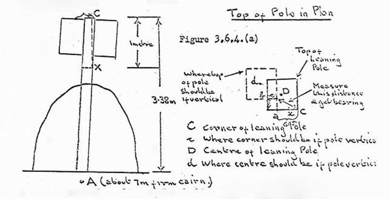
3.7. Plumbing Towers, Tripods and Beacons.

3.7.1. Towers.

These can be plumbed quickly and accurately over the station mark, with two theodolites. When engaged on tower work, it has been found necessary to carry an extra theodolite with the party erecting the towers.

The following method was adopted:-

See that the adjusting slot on each tower leg is approximately central on the bolts, so that adequate adjustment is available.

Set up the two theodolites about 120° apart, so that they can sight the station mark centrally between two tower feet. They should be about 30 metres from the tower.

Clear bushes, grass etc., so that the station mark can be seen - set match in the centre of the mark.

Level the theodolites, lay on station mark with both instruments and elevate them until they are laid on the tower head.

Look through theodolite No 1 first; loosen retaining bolts on tower foot opposite No 2 theodolite; move tower until the theodolite retaining bolt in the tower head, is cut centrally by the vertical graticule, in the theodolite telescope; tighten retaining bolts on foot opposite No 2 theodolite.

Look through theodolite No 2; repeat operation as above this time adjusting with foot opposite No 1 theodolite; as this is opposite theodolite No 1, this adjustment will not greatly move the tower off line, from that instrument.

If necessary, readjust for instrument No 1, tighten retaining bolts and lock. Do likewise for instrument No 2.

Remember all adjustments are done at the foot opposite the instrument to the one through which the tower head is being viewed.

3.7.2. Plumbing tripods or beacons.

Tripod, or quadrupod beacons, where the station mark is accessible would need to be plumbed as in 3.7.1., if observations are to be done to the vanes.

If observations have already been taken, the reverse method will have to be used; i.e., lay on centre of vanes from two positions, depress telescope, and mark plumb point on the ground, near station mark. Measure distance vanes off line, and take magnetic bearing. Draw plot to scale, showing the above details; calculate the eccentric correction as in 3.6.3.

Where lights are used and are plumbed over the station mark, naturally, the above does not apply.

3.8 Sigma Octantis Azimuth determination

3.8.1 Single-ended azimuth determinations, consisting of one set of 6 rounds, shall be observed on the terminal leg of every spur traverse, in a control survey. Additional azimuth determinations may be observed at any stage, to check the "carried through” geodetic azimuth.

3.8.2 Simultaneous reciprocal azimuth observations, consisting of two sets, shall be observed on specified lines, as required. They do not demand exact simultaneity of pointings by each observer. However, it is important that the two observers, at each end of the line, commence observing at almost the same time, and finish the two sets, within 10 minutes or so, of each other.

Figure 3.8.8

3.8.3 Main equipment necessary

Theodolite and lighting set

Radio, capable of receiving WWV or VNG.

Split hand stop watch

Pocket-watch with second sweep hand.

Observing screen or tent.

Booking lamp.

Torch (for reading plate bubble and stop watch.)

Lucas lamp and battery.

Traeger Transceiver for inter-communication with distant station.

3.8.4 Time of observation

Observations should commence immediately after sunset, or as soon as Sigma Octantis is visible. This is the most accurate period in which to observe, the RO light being at its steadiest at this time.

3.8.5 Light from RO

A Lucas Lamp, or other suitable light will be used. It is important, particularly in flat terrain, to keep the lamp as high above the ground as possible. The lamp should be plumbed over the station mark, if possible. If observations are also in progress at the station, the light should be placed exactly on line to the distant station with the theodolite.

3.8.6 Preparations for Azimuth observing

The zenith distance and azimuth of the star, to the nearest 2 minutes of arc, is calculated for the approximate start time of the observation. This is done on the graph, Figure 3.8.

Before consulting the graph, it is necessary to calculate the Local Sidereal Time at which it is desired to commence observations.

To compute Local Sidereal Time :

At NM/E/110 Latitude 26° 08', Longitude 132° 30'

Time, 1950 hours, Central Australian Time, on 1 March 1970

-west )

L.S.T. = R + U.T. +east ) Longitude

h m

Central Australian Time 19 50 (Time to nearest minute.)

09 30 East of Greenwich – 09h 30m

Universal time 10 20

R for 10h 20m U.T 10 35 (Pg 6 Star Almanac)

Longitude (East) 08 50 (132.5° Long in time /15)

29 45

-24 00

Therefore L.S.T is 05 45

3.8.8 To find zenith distance and azimuth of Simga Octantis

Using the computed L.S.T., the graph is used to find DH, and the azimuth of the star. DH is applied to the co-latitude, either positively or negatively, to give Zenith Distance, depending on whether the star is in upper or lower transit. In the example the correction is positive. Figure 3.8.8.

3.8.9 Setting the watches

The pocket watch should be set about 10 seconds fast, on Standard Time. The stop watch should be started at a suitable time, i.e. if a 30 minute dial, at 00 or 30 minutes, if a 15 minute dial, at 00, 15, 30 or 45 minutes. It should be started, within 1 or 2 seconds, of the same reading as the pocket watch. This means that both watches are about 10 seconds fast on Standard Time, and therefore any errors are more easily detected. The stop watch should be compared with the WWVH, WWV, or VNG time signal, noting the error to the nearest 0.10 second, just prior to the commencement of the azimuth observations, and also after half the observation has been completed, and at the conclusion of the observation.

3.8.10 Sequential Description of the Observing Method

After checking that the theodolite has been carefully levelled, parallax eliminated, focus adjusted, and the lighting in the telescope and circles suitable, then:—

(a) With the theodolite FL, take 2 pointings, and 2 micrometer readings on the RO light, in the same manner as for horizontal angles.

(b) Set-the zenith distance, and horizontal angle of the star, as called out by the booker.

(c) Adjust the vertical pointing of the telescope, so that the star appears just clear of the horizontal wire, and bring the star centrally between the 2 parallel vertical wires, calling "up" and pressing the stop watch button at that instant. On the call "up", the booker records the time indicated by the pocket watch.

(d) The observer calls out the stop watch reading, and the plate bubble readings, East and West, in that order.

(e) The observer calls out the horizontal circle reading.

(f) Take another pointing and micrometer reading, again reading the stop watch and plate bubble.

(g) Call out the horizontal circle reading; on this occasion read the vertical circle to the nearest minute, and call it out.

(h) Change face on the star. The booker will call out the vertical and horizontal circle settings, if desired by the observer.

(i) Take 2 more pointings and bubble readings, etc., on the star as before.

(j) Take a vertical circle reading, to the nearest minute of arc, on the star, after the second pointing.

(k) Swing back on the RO light and take 2 pointings and micrometer readings. This completes 1 round.

(l) The instrument should be relevelled after each 3 rounds. However, if at any stage it is noticed that the instrument is badly off level, it should be relevelled before commencing the next round from the RO.

(m) When observations are complete, compare the stop watch readings with the coarse readings of the pocket watch, looking for 30 second discrepancies. Reduce the field book as shown in Figures 3.8.10(a) & (b).

3.9 Hints on Ex-Meridian Sun Observation for Azimuth: Method and Booking.

(a) Time to observe

The best time to observe, i.e. when any error in Declination, Altitude, or Latitude will have least effect on the computed result, is when the sun is on or near the Prime Vertical, either East or West, and at an altitude of 20° to 30°.

However owing to the sun's path through the changing seasons, it will frequently be impossible to fulfill the above conditions. For example, in mid-winter, in Latitude 40⁰ (just south of Victoria), observations between 0930 - 1000 hours, and 1500 - 1530 hours EST will only give altitudes of from 17^° to 21^°, and bearings of approximately 40^° or 320^° which are well away from the Prime Vertical.

Obviously a compromise is necessary, and the observer must decide on a time to suit the time of year and the locality. Luckily, as the observer moves north in Australia and the Latitude becomes smaller, the conditions for the shape of the astronomical triangle improve for ex-meridian sun observations.

(b) Observing technique

As the tabulated values of Declination and "R" for the sun are referred to its centre, the observations are arranged in such a way that the mean of the Face Left and Face Right pointings will give an observation to the sun's centre. Observations are on the limb of the sun. Remember, in the morning the sun will appear to be descending, and in the afternoon it will appear to be ascending. Figures 3,9,(a) and (b) show the technique.

Initial location of the sun in the telescope.

The sun can blind if the observer forgets to fit the sun filter to the eyepiece end of the telescope.

To avoid danger from this, the following method of locating the sun, is recommended:-

(i) Standing beside the instrument, bring the shadow of the foresight onto the rear sight; lock the horizontal clamp.

(ii) Hold the palm of the hand behind the eyepiece, move telescope vertically until the image of the sun shows on the palm; lock the vertical clamp.

(iii) Immediately, slip the sun filter onto the eyepiece end of the telescope.

Laying on the sun

Experience has shown that the best method or laying on the sun is to use only one tangent screw to keep one limb of the sun on the appropriate crosshair, letting the sun's own movement bring the other limb onto its appropriate crosshair. When viewed through the sun filter the crosshair is only clearly visible against the bright disc of the sun, therefore the crosshair is initially laid close to the edge of the sun as shown in the first position in figures 3.9.(a) and (b).

It is then easy to concentrate on the diminishing-gap between the crosshair and the limb while still keeping the other limb on its crosshair with the tangent screw. The method can be clearly seen in the following

FL on RO 00° 00’ 30” approx )

Attach Sun Filter FL on Sun )

Change face FR on Sun ) 1 round

Remove Sun Filter FR on RO 180⁰ 00^’30” approx )

The second round commences with FR on the RC; leave scale setting as set, but re-lay on the RO, once again following the above sequence.

At least 4 rounds, possibly 6, are taken. Figure 3.9.(c) page of F.B.

(d) Additional data required

Time : Should be booked to the nearest second. Watch should be checked against a radio time signal; correct the booked time, if necessary.

Temperature & Pressure : Readings should be taken for use with the Refraction Tables. Those in the Chambers are based on a standard temperature of 10^°C, and a standard pressure of 754mm (1005.25mbs). Where observations are taken under conditions differing considerably from standard a noticeable error is introduced if actual readings or both temperature and pressure are not used in the computation.

Refraction taken from Chambers is multiplied by:

(Actual Pressure (millibar) ) * ( 283 )

(1005.25 ) (273 + Actual T°C )

Refraction increases as pressure increases BUT decreases as temperature increases.

The back page of the Sun Observation reduction proforma has refraction and parallax tables for the sun based on zenith distance.

The Refraction Table is based on 57”*tanZD

The Parallax Table is based on 8.8”*sinZD.

Plate bubble : Usually,with a sun observation for azimuth, it is not considered necessary to record, and correct for, any dislevelment shown by the plate bubble. However, it must be emphasised that if great accuracy is the aim, any dislevelment of the horizontal axis must be taken into account.

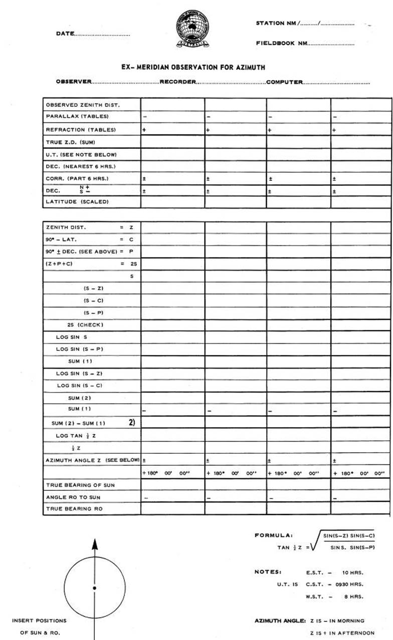
3.9 Sun observation for Azimuth – Hour Angle and Accurate Time

Traditionally, the method used for observing the sun for azimuth has been as previously described, i.e., reading simultaneously the altitude and the horizontal angle to a reference point using time within one minute. As this method requires no sophisticated equipment and only an accurate Latitude, it is not surprising that it became the method almost exclusively used.

The main drawback to this observation is the limited time each day that the sun is in a suitable position, and the time necessary for the observer to become proficient in the technique of simultaneously pointing to both the horizontal and vertical limbs of the sun.

It is pointed out by Dr. G. Bennett of the University of NSW in an article in "The Australian Surveyor", March 1974, that the Hour Angle method using accurate time is now well worth considering because:-

(i) Time signals from VNG should be audible over most parts of Australia during daylight hours.

(ii) Small transistor short wave radios for receiving these time signals are readily available.

(iii) Split hand stopwatches are also readily available.

(iv) Current map coverage is such that Longitude can now be scaled as accurately as Latitude.

(v) The method permits the surveyor to take observations over a greater time range, (even observations at noon, in the winter months should be quite satisfactory.)

(vi) The observer has only to concentrate on laying on the vertical limb of the sun and reading the horizontal angle.

(vii) In an observation where speed is essential, considerable time is saved in not having to adjust the alidade bubble and read the vertical angle.

Setting the watches and Time Signals

The procedure laid down in 3.8.9 should be followed, however it should be emphasised once again that accurate time is critical in this observation therefore care must be taken to rhythmically "beat" the stopwatch in unison with the "beep" of the radio signal. Beat the finger on the stopwatch button a number of times until this slight sound is synchronized with the "beep" of the radio time signal. Once this is achieved press the button on one of the "beeps". Do not "snatch" at the button on this "beep" or good synchronisation will be lost; this is a common fault while learning.

The mean of at least five synchronizations should be taken. Unless cloud causes delay, the sun observation is finalized quickly; where this is the case a time signal check immediately prior to and immediately following the observation is sufficient. Where delay occurs take farther time checks during the waiting period.

Observing and booking

Reading the stopwatch and recording the observed data is similar to that of the Sigma Octantis observation for azimuth except that the plate bubble is not read and no vertical angle is required. As the altitude of the sun is not observed, temperature and pressure readings are not required.

The example in Figure 3.9(d) shows the booking method using the same field book page as for the Sigma Octantis observation. It is advisable for the observer to call out each vertical limb of the sun as he lays on it; the booker can record this in the Vertical Circle column as shown. This procedure should ensure that the observer does not forget to change to the opposite limb of the sun as he changes face. The observation in the example was done using single pointings, however any observer, once he has attained sufficient speed, would be advised to use the double pointing method for greater accuracy and less chance of gross error.

The computation of this observation is shown in Figure 12.7(3), Volume 2 of these notes.

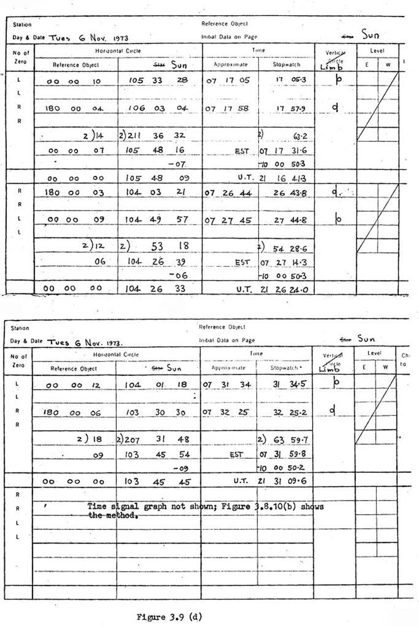
3.10 Meridian Transit Observations for Latitude & Longitude – Rimington’s Method

A method of astronomical observations for Latitude & Longitude was needed mainly to provide control for minor traverses in the N.T. and also the 4 mile map series owing to the fact that little triangulation control was available at that time (1940-1955).

To make the observation an economical proposition the requirements were:-

(a) Observations for both Latitude & Longitude needed to be done on the one night and take no more than a couple of hours.

(b) Field computations to prove that the result was acceptable had to take no more than about the same length of time, so that they could be done on the same night or first thing next morning, to enable the observer to move on (unless, of course, the computations indicated further observations were necessary).

After considerable research, the following method was evolved by Mr. G.R.L. Rimington. His paper in the Australian Surveyor, combines a description of the method and the calculations necessary, with the historical background of the first trial observations.

The following is a brief description; this is then amplified in a "step by step" procedure.

(i) A programme of stars is prepared.

(ii) Theodolite is laid out on a N-S line, stars are paired alternatively N & S, or vice versa.

(iii) The accurate time and "rate” of the chronometer is found; it is advisable, but not necessary, for the chronometer to be slightly fast, and it is probably best set on the standard time of whichever Australian Time Zone the observer is in. However, it can be set on GMT (UT), if preferred.

(iv) Longitude observation. Using the "early stadia" wire, the star is timed on FR by stopwatch and chronometer prior to its reaching the centre wire (the meridian), and timed again, this time on FL as it reaches the same "offset" wire, now termed "late stadia". From this it can be seen that the star is not timed as it crosses the meridian, the time that this actually took place being the mean of the "early" and "late" stadia times.

(v) Latitude observation. As the star crosses the meridian (centre wire) on FL, the vertical angle is read. This is the Z.D. with the Wild T2.

(vi) The above procedure is repeated with a star in the opposite direction to give a "pair". Computation of this pair will give both a Latitude and Longitude of the position.

The observation needs no elaborate equipment; the main requirements are :

(i) Theodolite, Wild T2, or similar, with Talcott Bubble if possible. Also lighting set, prismatic eyepieces and tripod. The instrument to read to one second, the telescope to elevate to about 70°, and to have two, "offset" vertical hairs. The instrument selected was the Wild T2, and the two "offset" vertical hairs were placed at the same distance L & R of the centre vertical wire as the normal stadia wires are above and below the horizontal wire, i.e., about 17 minutes of arc. Thus the names "early Stadia" and "late Stadia" have been adopted for these two hairs. See Figure 3.10(a).

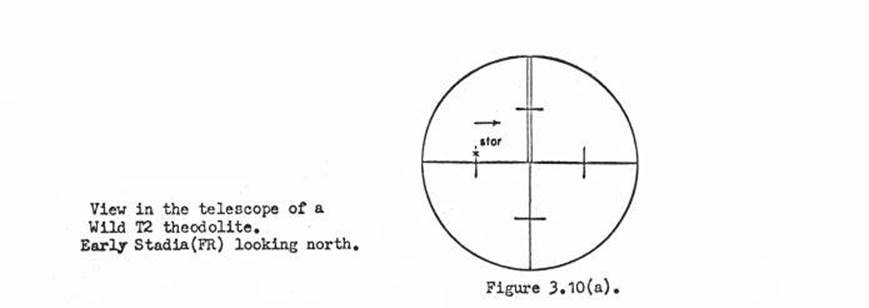
(ii) Surveyor’s or ship's chronometer, half second beat. Good stopwatch reading to one-tenth of a second, with wide enough graduations to estimate to one-hundredth of a second, pocket-watch.

(iii) Apparent Places of Fundamental Stars (FK4), star programmes, Sigma Octantis graph, field books, maps, etc.

(iv) Table and light for booker, thermometer.

(v) Observing pegs for theodolite tripod.

For this observation there are four main steps :

(i) Office preparation of a star programme and the Sigma Octantis graph.

(ii) Field preparations before dark

(iii) The actual observation after dark.

(iv) The field computation before leaving the station.

Step 1 Office preparations

(a) Programme of stars

Once the general area for the field work is known a programme of stars is prepared for the Mid-Latitude of that area. A long list of suitable stars is extracted from the FK4. They are listed as North or South, Name, Magnification, RA & Dec, and columns are left in which to enter (360°-ZD) and ZD, on arrival at the place where the observation is to take place.

The RA is not listed as such but as "Early Stadia", and a time allowance of approximately two minutes to the RA is made to allow for the difference in time between the stars arrival on the "Early Stadia" and its arrival on the centre wire (the meridian).

As the North stars move a lot faster than the South stars, it is worth calculating this time allowance for both North & South stars of a suitable ZD for observing. This can be done thus:‑

The value of the space between the stadia Wires is 1:100 which is 34' of arc (2.26 minutes of time). Thus from a stadia wire to the centre wire as 17' of arc (1.13 minutes of time).

This time interval x Secant Declination of the star gives the time the star will take to travel from the stadia to the centre wire, (or stadia to stadia, if required).

A North star with a Sec. Dec. of 1.0610 x 1.13min = 1.20min. Therefore "Early Stadia" for this star is RA -1.20min, allow 2min.

A South star with a Sec. Dec. of 2.0050 x 1.13min = 2.26min. Therefore "Early Stadia" for this star is RA-2.26min, allow 3min.

The above figures are approximate only; as no correction has been made for Latitude, they apply to a point on the Equator.

This can be used also to check doubtful observations, and is an indication of the time available for changing face and reading the ZD as the star crosses the centre wire. When checking doubtful observations always allow for the Latitude.

Diagrams for 30° South Latitude

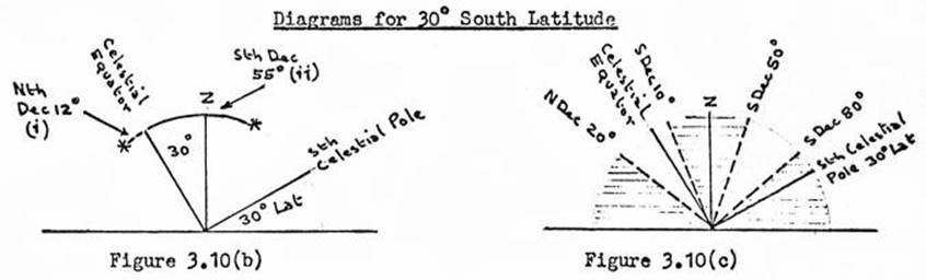
(i) Star with Nth Dec. of 12° would have a ZD of 30° + 12° = 42°. It would be to the observers north and would be O.K.

Stars in the shaded area are unsuitable, thus stars with North Dec. of 0° to 20° & South Dec. of 0° to 10° are suitable North stars. Stars with a South Dec. between 50° & 80°, are suitable South stars

(ii) Star with a Sth Dec. of 55° would have a ZD of 55° - 30° = 25°. It would be to the observers south and would be O.K.

In selecting stars for the programme, list those between about 1.0 and 6.0 magnitude. Use in the observation, wherever possible, those between 2.5 and 5.5. As the Wild T2 will only elevate to about 70 (20° ZD) and because of greater unreliability of refraction in lower altitudes, stars with a ZD over 50° should not be selected, another limitation is placed on the stars which can be entered in the programme. Draw rough diagrams as in Figures 3.10(b) & 3.10(c) to give a clear picture of the stars which can be selected.

The selected stars for a six to seven months observing season cover about three foolscap pages and will be useable for some years. Sufficient copies to permit the using of one programme per station should be made available to each observer.

A computer programme is now available to select stars for such a season’s work.

(b) Graph for the location of Sigma Octantis

A graph giving the ZD and Azimuth of Sigma Octantis at any LST at the Equator should be made.

For the accuracy required there is no need to solve the astronomical triangle; just use a series of plane triangles with the hour angle each half hour between 0hr and 06hrs and the hypotenuse the CO - ZD (Polar Distance). Thus the Polar Distance x sine hour angle gives the Azimuth correction, and the Polar Distance x cosine hour angle gives the ZD. See Figure 3.10(d).

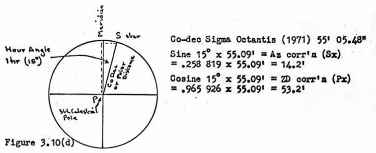
As the RA of the star is the LST when the star is on the meridian, this is the start point for the graph, points are plotted to obtain both ZD and Azimuth curves for each half hour from this start point. Thus in 1971, with the RA and Dec. of Sigma Octantis 20h 40m 04.36s and S89° 04' 05.48² respectively, 10 right angled triangles with the hour angle each half hour (in arc 7.5°) increasing from 7.5° to 82.5°, and with the hypotenuse (Co-dec.) a constant, can be quickly solved on a calculating machine. Signs for these corrections are indicated in Figure 3.10(e).

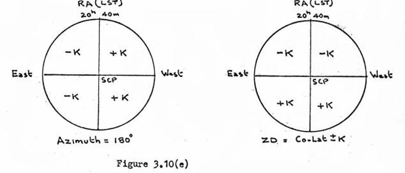
There is a slight variation in the movement of Sigma Octantis from year to year; while this is not sufficient to cause trouble in locating the star, if it is required to use the graph to lay out on a reasonably accurate azimuth, the graph should be recalculated each couple of years. Figure 3.10(f) shows one form of this graph while another type is shown in the chapter "Sigma Octantis azimuth determinations", Figure 3.8.

Step 2 Field Preparations

Setting up

The following requirements must be satisfied:-

(i) The instrument must be oriented with two footscrews along a N-S line so that the instrument can be levelled in the plane of the meridian and across the plane of the meridian. Keeping the instrument perfectly level across the meridian is vital to the accuracy of the longitude part of the observation.

(ii) The vehicle should be positioned so that it protects both the theodolite and the booker from the wind, and is close enough to satisfy the next step.

(iii) The booker's table, on which the chronometer will be placed, must be positioned within 3 paces of the theodolite and beside the vehicle. The chronometer must be placed so that the observer can get to it without stepping over a tripod leg.

(iv) All usual precautions in setting up the theodolite for accurate work must be taken.

(v) Booker prepares his set up.

Figure 3.10(g) shows a good lay-out.

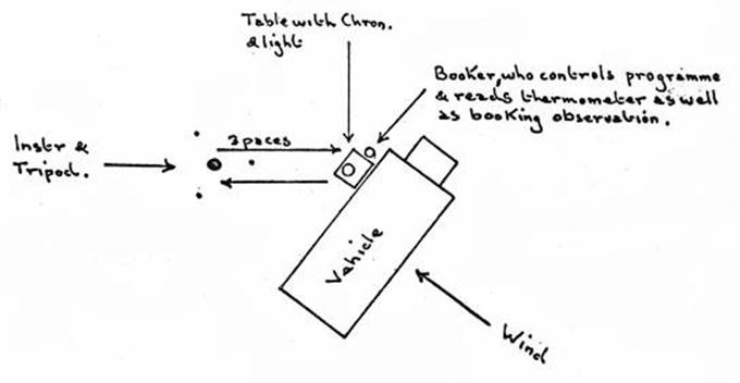
(b) Preparations before dark

(i) Scale from the map, the Latitude & Longitude to the nearest minute. Decide on the time when Sigma Octanis should become visible and calculate the LST at this time:‑

LST for 1900hrs WST on 1/3/71. Latitude 29°08'. Longitude 127° 16¢.

WST 19 00 00

minus zone 08 00 00

GMT (UT) 11 00 00

+ Sidereal Correction 01 49

+ Longitude in Time. (127° 16' /15) 08 29 04

+ Sid. time at 0hrs UT, 1/3/71. 10 32 35

30 03 28

-24h gives LST 24 00 00

06 03 28

From the Sigma Octantis graph calculate the ZD & Azimuth of the star at the above LST. At 1900 hours the booker should start the pocket watch at this LST (nearest minute.). The fact that the watch is running at mean time rate does not matter over the short period between the time the watch is started and the conclusion of the observation.

(ii) On the observing programme, fill in the ZD & (360°—ZD) of each star which it is intended to use and bracket them in "pairs" North and South; make sure a surplus of stars are ready in case of delays. From Figure 3.10(h) the procedure is evident.

The selection of pairs is a matter of compromise, but the difference in the ZD's should not generally exceed 10°. The stars magnitude should generally range between 2.5 and 5.5 for easy intersection.

The observer may at times have to observe outside these limits. However, it is generally found that stars brighter than 2.5 are too large to intersect easily & accurately, while those smaller than 5.5 are not easy to see. The clarity of the night will also effect this; on a very clear but moonless night, stars in the vicinity of 6 magnitude may by intersected quite easily, while on quite a few cloudless nights there is sufficient "murk” in the air to make stars which would normally be quite bright, appear very faint. Therefore these stars become the only ones suitable for observations on this type of night.

With the ZD's of the stars, remember that the higher they are in the sky, the less they will be influenced by refraction, thus the aim is to use N & S stars of almost similar ZD's and as near the highest altitude the instrument is capable of as is possible.

Obviously a N star with a ZD of 20° and a S star with a ZD of 60° do not make a good pair as they rely too much on something which is impossible to calculate accurately, i.e., refraction.

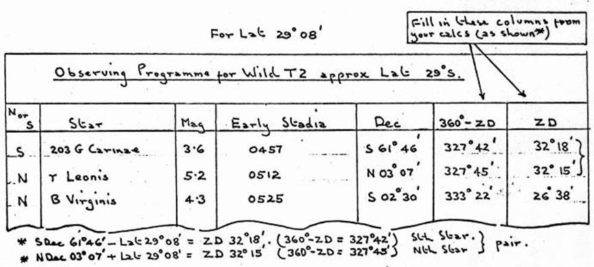
(iii) As darkness closes in, the telescope and graticule focus are adjusted by sighting on a bright star and "taped" with Durex to prevent movement during the observation. The same thing applies to the micrometer telescope. The reasons for this are fully explained later in the "Method of Observation". The theodolite should now be levelled using the "Talcott" bubble and then laid out on an approximate N-S line with a prismatic compass, taking into account the Mag. Declination.

(i) Time signal check

Obtain a time comparison on VNG, the Australian P.O. time signal station at Lyndhurst, Victoria. (See Annexure C of "Specifications for Ground Control Survey" for details of this and other time signals.) Check the minute and second for gross error on WWVH (or WWV).

If unable to receive VNG, use WWVH (or WWV) and check minute and second with the hourly ABC time signals.

Obtaining accurate time is entirely a matter of constant practise in achieving a rhythmic one second beat of the finger on the stopwatch button. Hold the stopwatch with the index finger lightly pressing on the stopwatch button; beat with an up and down motion of the hand until the beating of the hand and finger is in unison with the beat of the time signal. Once this synchronization has been obtained, press the button on the stopwatch. Do not "snatch" the button on this beat thus taking a decimal which can be widely in error. This tendency to "snatch" and thus press the button too early is very noticeable in the learner. A good quality stopwatch, the second divisions of which are wide enough apart to estimate the "hundredths" is necessary.

Step by step procedure for taking time signals.

1. Switch on the radio, beat watch until in unison with the second beat on the radio.

2. Switch off radio and go through the same procedure with the chronometer. As the chronometer beats half-seconds make sure that synchronization is made on a full second beat. About 10 of these comparisons must be made; the mean of all these is recorded as the decimal of the second. Record two places of decimals.

3. About 5 seconds before any 5 minute time signal start to beat the watch and on the exact five minute signal press the button to start the watch.

4. Switch of the radio, beat until in synchronization with the chronometer, then stop the watch on a ten second division on the chronometer. It must be remembered that with VNG, WWVH & WWV, the 59th second of every minute is not sounded therefore care must be taken to start beating the watch at about the 54th or 55th second so that coincidence with the time signal is obtained by the 58th second and kept over the missing 59th second to ensure there is good synchronization when the button is pressed on the 60th second.

5. Write down the second and decimal reading on the stopwatch and the chronometer. In the stopwatch reading replace the decimal with the decimal obtained in step 2, i.e.; if the single reading on the 5 minute is 17.8s, and the mean of the 10 readings was 0.93s the booked stopwatch reading is to be 17.93s not 17.8. Thus if the chronometer read 19h 20m 50s and stopwatch read 17.93s at 19h 20m 00s, the chronometer is fast:-

Chronometer reads 19h 20m 50s

Stopwatch reads 17.93s

Chronometer time (when time signal taken) 19 20 32.07s

WST (when time signal taken) 19 20 00

Chronometer fast 32.07s

Always take a second time check to ensure there is no mean error of one or more seconds. If using VNG check with WWVH or WWV, or if using either of the latter stations, check with the ABC on the hour.

(ii) Locating Sigma Octantis using the graph

Just prior to 1900hrs, set the calculated ZD of the star on the theodolite and commence searching East and West of the approximate meridian until the star is identified. The ZD is the main factor in locating the star as the Latitude is normally known fairly accurately therefore the ZD interpolated from the graph should bring the star fairly close to the horizontal cross wire.

(iii) Final check of level

Having located the star and before laying the theodolite accurately on the meridian, it is best to finally level the instrument as it probably may have been moved off level while searching for the star. Level first with the two footscrews along the meridian, then with the single footscrew across the meridian. In future relevelling, as the level along the meridian is not so critical it need only to be done carefully at the present juncture, unless the theodolite is accidently knocked when complete relevelling would be necessary. If the star was located quickly and easily, leaving the observer confident he has not moved the level of the instrument, he may prefer to lay on the meridian, then just touch up the level before commencing the observation.

(iv) Laying the theodolite on the meridian

Now calculate the ZD and Azimuth of Sigma Octantis for a convenient LST a few minutes ahead, and intersect the star between the double wires, at that instant. Once the star has been intersected, set the calculated Azimuth on the horizontal circle. Turn the theodolite to 00° 00' 00" (if a North star is to observed first) or 180° 00' 00" (if the first star is to be a South.) Make sure the micrometer drum has been turned to 00' 00". The theodolite is then assumed to be in the plane of the meridian and all preparations for the observations have been completed.

The actual observation

Notes :

(a) The calculated values (360°- ZD) & ZD on the programme refer to the vertical circle setting of the Wild T2 theodolite FR & FL respectively. If another type of instrument, graduated differently, is used these values will have to be adjusted to suit.

(b) As the prismatic eyepieces are only screwed in by normal thread, a drill for reversing them must be adhered to during the observation. Otherwise they may be screwed either right out (and fall on the ground), or right in (and cause the focus to be altered). Therefore prior to plunging the telescope, turn the eyepieces one half turn out when changing from FL to FR, and one half turn in when changing from FR to FL.

(c) Except when actually reading the ZD of a star, the micrometer drum must always be set at, and remain at 00' 00". If this procedure is followed the possibility of error in setting on the meridian will be eliminated, as the theodolite has to be laid on the meridian a minimum of 10 times during the observation, and speed is essential, any safeguard is important. Remember, at all times, that the horizontal circle itself is the R.O. for orienting the instrument.

Step by step procedure

1. As the theodolite is laid out on the meridian the first star of a pair is selected. If the star is to the North, the instrument will be laid out at 00° 00' 00", and if the star is to the South, it will laid out at 180° 00' 00" on FR, in both cases.

2. Set the programmed 360°- ZD on the vertical circle, always estimating the minutes. A few minutes before the programmed Early Stadia time, watch for the star to appear. Check the identity by the star's magnitude and time of appearance. With the vertical tangent screw bring the star to a position where it moves across the diaphragm, just slightly above or below, the horizontal wire. See figure 3.10(a).

3. At the instant the star cuts the Early Stadia wire press the stopwatch button.

4. Move to the chronometer, beat the watch until in rhythm with the beat of the chronometer and stop the watch on a 10 second division of the chronometer.

5. Call to the booker this chronometer time in the order, seconds, then minutes, then the hour, and lastly the stopwatch reading. The assistant should repeat these readings as he books them; also read and book the thermometer value.

6. Return to the theodolite, reverse the eyepieces, plunge the telescope, change to FL and lay on the meridian at 180 00' 00" (North star) or 00° 00' 00" (South star).

7. Set the programmed ZD on the vertical circle, again estimating the minutes. Identify the star, and when it is near the centre wire intersect it on the horizontal wire.

8. Bring the ends of the alidade bubble into coincidence, bring the vertical circle graduations into coincidence with the micrometer drum, call out the ZD reading, the assistant repeating it back as he books it. Reset the micrometer drum to 00' 00".

9. Move the star slightly off the horizontal wire and at the instant it intersects the Late Stadia, press the stopwatch button.

10. Again move to the chronometer, beat the watch until in rhythm with the beat of the chronometer, then stop the watch on a 10 second division of the chronometer.

11. Again call the readings to the assistant as in step 5, this time there is no need to read the thermometer.

The above steps complete one star; proceed similarly with the other star of the pair. Five good pairs are necessary, but if in doubt of the quality of any observations, take an extra pair or two.

Relevelling between pairs of stars

Relevel, across the meridian with the single footscrew, between each pair of North and South stars which form a complete observation. Remember that the quality of this observation depends entirely on keeping the vertical axis of the instrument truly vertical, particularly across the meridian and bearing in mind that during a period of 20 or more minutes, it is exceedingly unlikely that the instrument will remain truly level.

Time check in the middle of the programme.

Always obtain a time check somewhere near the mid-point of the observation, say, after the third pair. This is necessary to see if the observer is consistent in his time-keeping, or whether the chronometer has an uneven "rate".

Time check after completion of the observing program - Drawing time graph

The final time check should be made immediately after the last star has been observed. Plot a graph showing the times fast or slow against the chronometer times at which each time signal was taken. Draw a “line of best fit" between the three plotted points to obtain a graph from which can be read the varying amounts that the chronometer is fast or slow at the times which each star was observed. The station number and date is noted against this graph.

The observation with a split-hand stopwatch.

To avoid having to carry a chronometer this observation could be done with a good quality split-hand stopwatch and using a pocket or wristwatch for rough times.

This system would be ideal for any field party which is only required to observe an occasional astrofix among its normal duties. Naturally, if the party's full time task was the astrofix, a chronometer would be more satisfactory. Full details for using the split-hand watch for Azimuth observations are given in 3.8.10. When observing for Latitude and Longitude these lines would be followed except that the time check procedure must be adapted to ensure very accurate times.

As well as the full time checks prior to and after the observation, a time check for the second and decimal (to hundredths) would need to be taken immediately before and immediately after, each pair of stars. This is for the decimal and second only, the other checks taking care of the minute and hour. This check can be done quite quickly, however the delay may cause the observer to miss some stars he would normally use; even so the full time of the observation should not be beyond that which is acceptable.

Computation

The calculation of the Latitude and Longitude from this observation is dealt with in 12.10.

3.11 Tacheometry or Stadia Surveying

Stadia provides a method of measuring distances and differences of elevation by merely sighting a staff. This can be done with a level or an orthodox theodolite providing the instrument has two horizontal crosswires, called "Stadia Wires", at equal distances above and below the central horizontal crosswire. These stadia wires are so arranged that the "intercept" (the distance between the two staff readings, as read against each stadia wire and usually called "S") is 1/100th of the distance, instrument to staff, when the line of sight is horizontal and the staff is truly vertical. See figure 3.11.

The level is mentioned only in passing, these notes henceforth will deal with tacheometry where the line of sight may be inclined and where horizon angles or true bearings will be required.

When the line of sight is inclined, the intercept is multiplied by appropriate factors, depending on the angle of inclination; the results give the horizontal and vertical distances from the point on the staff cut by the central crosswire, to the axis of the theodolite.

It will thus be seen that the bearing, distance and level of a point can be obtained in one observation.

3.11.1 Theory

As shown in figure 3.11.1, the vertical angle, a, and stadia intercept DE (or S) have been read; required are AB (the horizontal distance) and BC the vertical distance between the axis of the theodolite and the central reading on the staff.

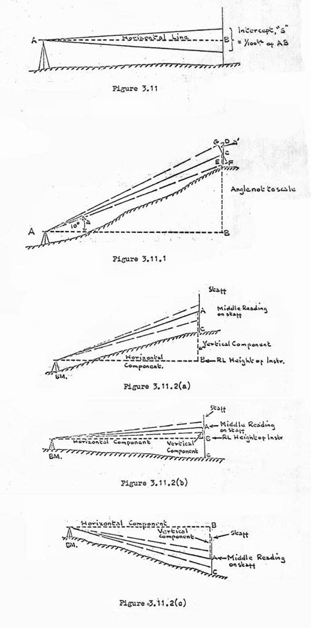
Step 1

The intercept on the staff DE, has to be turned into a distance GF, which is a line perpendicular to the line of sight AC. The vertical angle “a”, is equivalent to “a'”, therefore DE x cos a' = GF. In the example DE (or S) = 4.21 and “a” = 10°, therefore 4.21 x .984 =4.146.

Step 2

With stadia 1 to 100, AC = 100 x 4.146 = 414.6.

Step 3

Solving the triangle ABC for the horizontal distance AB, 414.6 x .9648 = 408.30.

Step 4

Solving the triangle ABC for the vertical distance BC, multiply AC by sine 10°, that is 414.6 x .17365 = 71.995.

The above is normally shortened to:

AB (the horizontal component, known as H) = 100S cos² a, and,

BC (vertical component, known as V) = 100S sin a x cos a or

= 100S ½sin 2a.

Thus to obtain the H & V components of the sighting, the intercept S, must be multiplied by the factors shown above. Tables are available for these and many slide rules have special graduations so that when the intercept on one scale is placed opposite the zero angular graduation the horizontal component appears against the observed vertical angle in the portion of the scale marked "H", and the vertical component appears against the observed vertical angle in the portion of the scale marked "V".

3.1.2 Reduction of Stadia Observations

Case 1:

Angle of Elevation with base of staff above Bench or Station Mark. As shown in Figure 3.11.2(a) the vertical angle is an angle of Elevation, and the base of the staff is above the BM. BM value + Height of Instrument = Reduced Level, height of Instrument.

The vertical component (AB in diagram) is now computed and is positive.

Add to R.L., height of Instrument to obtain R.L. of Middle Reading on staff (A in diagram).

To obtain R.L. of point C (Ground level at base of staff), subtract the Middle Reading on the staff from the RL of point A.

Case 2:

Angle of elevation with base of staff below Bench Mark or Station Mark. This can occur on slightly sloping ground where it has been necessary to elevate the line of sight to clear bushes, long grass, etc. The V.C. is computed and is positive. Add this to. R.L. height of instrument to obtain RL of Middle Reading on staff (A).

As in Case 1, just subtract the Middle Reading on the staff from the RL of point A to get RL of point C. Note that in this case the R.L. so obtained will be seen to be lower than that of the BM even though a vertical angle of Elevation was read. See Figure 3.11.2(b).

Case 3:

Angle of Depression. The V.C. is computed and is negative. Subtract from R.L. height of Instrument to obtain R.L. of Middle Reading (A).

To obtain the RL of point C, subtract the Middle Reading on the staff from the RL of point A. See Figure 3.11.2(c).

Formula:-

In all cases it is R.L. Stn B = R.L. Stn A.+ Height Instrument ± VC – MR.

In practise it is most convenient to evaluate ± VC – MR for each point, the result being called the "difference in elevation", then add or subtract this from the R.L. Height of instrument.

Equipment

Special theodolites and staves are available for Tacheometry work also levels which incorporate, a horizontal circle. However mostly an orthodox theodolite and staff will be used; these notes, therefore will be confined to such equipment. If one understands the theory and practise using this equipment, it is but a small step to change to more sophisticated equipment should the occasion arise.

3.11.3 A Detail traverse using Tacheometric Methods – Wild T2 or similar theodolite

The traverse would be through a line of main stations, picking up detail by means of subsidiary points along the traverse route.

Angular Work

The instrument should be checked to see that it is in good adjustment as it is customary when laying on subsidiary points to read both horizontal and vertical angles to the nearest minute on one face only, usually face left. Unless a higher degree of accuracy is required, the main traverse angles, both horizontal and vertical will be read to the nearest 10 seconds.

When the arc on Face Left has been completed, change to Face Right on the RO and read the main traverse horizontal and vertical angle only on this face. This helps increase the accuracy of the main traverse angles and is a check that the circle was not disturbed during the single face readings to the subsidiary points.

Reading the Staff

The staff must be equipped with a bubble to ensure verticality, and a check made to see that the bubble is in adjustment before the traverse commences.

The most simple method is to lay the bottom stadia wire on an even foot graduation on the staff, with the centre wire somewhere in the vicinity of 5 to 6 feet; i.e., approximately the same height as that of the theodolite.

Staff readings along the main traverse line are read twice, i.e. forward and backward, the distances and heights must be calculated in the field to check for gross error. Distances should agree within 1 foot and difference heights within 0.10 ft.

3.11.4 Field Book

There are various forms of field notes, That shown in Figure 3.11 is recommended for completeness and for clarity.

Column 1. The number (or name) of the station, RL station mark, height of Instrument.

Column 2. Sketch of the traverse legs and details of subsidiary points oriented on magnetic bearing.

Column 3. The station observed.

Column 4. The Horizontal angle observed.

Column 5. The Vertical angle observed; indicated positive or negative.

Column 6. The three readings on the staff.

Column 7. The "intercept", S.

Column 8. The calculated horizontal distance.

Column 9. The calculated vertical component, indicated positive or negative.

Column 10. The difference in elevation, indicated positive or negative (obtained from the algebraic sum of Mean Reading on staff & V.C.).

Column 11. The Reduced Level of the height of instrument; data from Col 1.

Column 12. The Reduced Level of the distant traverse station or subsidiary point; obtained from the algebraic sum of columns 10 and 11.

Column 13. Space for any necessary notes.

3.11.5 Errors caused by changing focus of the theodolite telescope

For internal focusing telescopes, which are the only type likely to be encountered, the factor D = 100 S, changes slightly with changing focus and varies slightly from instrument to instrument.

These variations are negligible except for very accurate measurements. For such determinations, it will be necessary to plot a correction curve for the instrument being used. The corrections are obtained by measuring exact stadia intercepts at various accurately measured distances; the following are recommended: 25, 50, 100, 200, 400, 800 and 1600 feet.

3.11.6 Accuracy

Horizontal Distances

An accuracy of about 1 in 1,000 would be about the best expected. The serious sources of error are in the measurement of the intercept and the verticality of the staff.

Errors arising from the measurement of the vertical angle and, the multiplying constants are negligible.

Heights

On a sight of 1,000ft, with a vertical angle of 6°, and allowing for a horizontal distance accuracy of 1 in 1,000, the error in the difference height could be about plus or minus 0.10ft; however with a sight of 500ft and a vertical angle of 1°, the error could be only about plus or minus 0.01ft. Therefore unless size of vertical angle and length of sight are taken into account, no figure for accuracy can be given. The following can be used as a guide :

For average length lines, (up to about 700ft) and with average vertical angles (up to about 5°) the best accuracy of difference heights between points would be about plus or minus 0.05ft.

3.11.7 Curvature & Refraction

The influence of curvature and refraction on heighting by Tacheometric means commences to show once sights reach 700 feet in length, where it is still only about +0.01ft. However, as it increases with the square of the distance, it becomes about +0.57ft at one mile (5280ft).

From these figures it can be seen that not a great number of sights will be affected. If the vertical angles on sights above 700ft are observed reciprocally, and the mean of such angles used curvature and refraction will be eliminated. This is the best method to adopt.

For further notes on curvature and refraction, including the calculations necessary to obtain the curvature and refraction for any line where angles have been observed from one end, only, see Section 12.4.

3.12 Almucantar observation for Longitude with Wild T3 Theodolite and stopwatch

For this observation, the instrument must be fitted with a graticule having 5 horizontal intersections on the vertical wire, each 5 minutes of arc apart (i.e. two above and two below the central horizontal cross-hair).

Also the alidade bubble must be graduated at approximately 2 mm intervals.

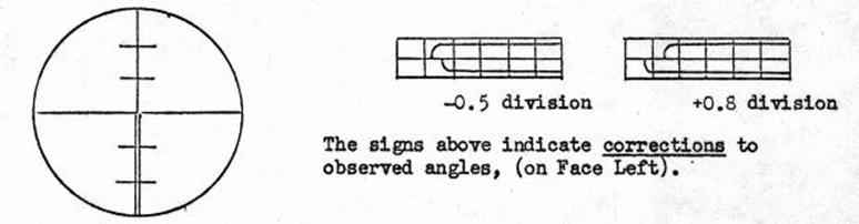
Graticule Alidade bubble graduations, Wild T3 on F.L.

Figure 3.12 (a)

Stopwatch

This must be of the split-hand type and be of good quality with a large dial, clear figures and graduated to 1/10 second; estimate to 1/100 sec.

Pocketwatches

An accurate Pocket or sweephand wrist watch is necessary. This watch must have the capability of the second hand "marking time" when the winding button is held out so that second and minute hands can be synchronised.

In addition another watch, or even an alarm or travelling clock is necessary as a "Prediction" watch.

Prediction Sheets

See Technical Report 4 for details of the preparation of Data Sheets for the electronic computation of Prediction Sheets for this observation with the Wild T3 theodolite.

The predictions are prepared for the approximate date that observations are to take place; in the Longitude programme each star is listed by Number, Magnitude, True bearing (nearest minute) and Time. The time is the standard time for the relevant time zone, i.e. in Australia EST, CST or WST as the case may be. If observations are not done on the exact date programmed, an allowance of 3.94 minutes (3 min 56 secs) per day must be made. That is, stars will be at the sane elevation 3.94 minutes earlier each day. This can be allowed for by pencilling in the correct time for the observing date or by setting a separate "prediction" watch to agree with the programme. If observations are later than the programmed date, the stars will be early therefore the watch must be set fast. See Figure 3.12 (b) for a prediction sheet, Wild T3.

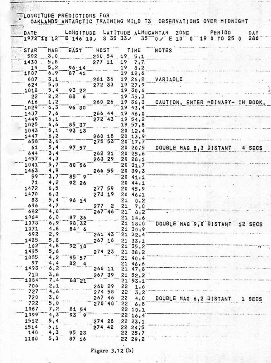
Radio

A good quality transistor radio with a short wave band capable of receiving WWVH or VNG (Lyndhurst, Victoria) is required. It should be noted that with the recent introduction of "atomic" time there will now be a correction, varying with the date, to be applied.

Number of Pairs

As distinct from the Latitude observation there is nothing to gain by selecting pairs in advance. Any East star can be paired with any West star, providing they are observed within twenty minutes of time. The aim should be 16 pairs, 8 on each of 2 nights; the minimum is 12 pairs with not less than 6 pairs on each of 2 nights.

Time Signals : setting the main watch and stopwatch

About 30 minutes before observations are to commence, but not on an exact hour or half hour, the main watch should be set by radio time signal, about 10 seconds fast. Take care to synchronise the minute hand and second hand or in other words don't have the second hand 10 seconds fast and the minute hand in a position which indicates about 30 seconds fast (or slow).

On the next even hour or half hour on this watch, the starting button on the stopwatch is pressed so that the stopwatch is started in syncronisation with the main watch. Lock the starting button of the stopwatch with a clip made from a "glider" clip. This will prevent the whole observation being wasted if the wrong button is pressed during the observation.

Beating the watch

The accuracy of the Longitude observation using a stopwatch is completely bound up in the observer's ability to rhythmically beat the stopwatch in unison with the "beep" of the radio time signal obtaining such consistency that the mean of his beatings will be close to 0.05 seconds plus or minus personal error. (See personal equation).

Much practice is needed and care must be taken to avoid making whole second or whole minute errors while concentrating on obtaining the accurate decimal of a second.

Beat the finger on the stopwatch button a number of times until this slight sound is synchronised with the beat of the radio time signal. Once this is achieved press the button on one of the beats. Do not "snatch" on this beat; learners tend to do just this after having got into a good rhythm. Thus having lost this rhythm on the final beat their result could be 0.1 second or more in error. The mean of 5 series of signals is taken, see Figure 3.12 (c) for an example of the time signal page of the field book.

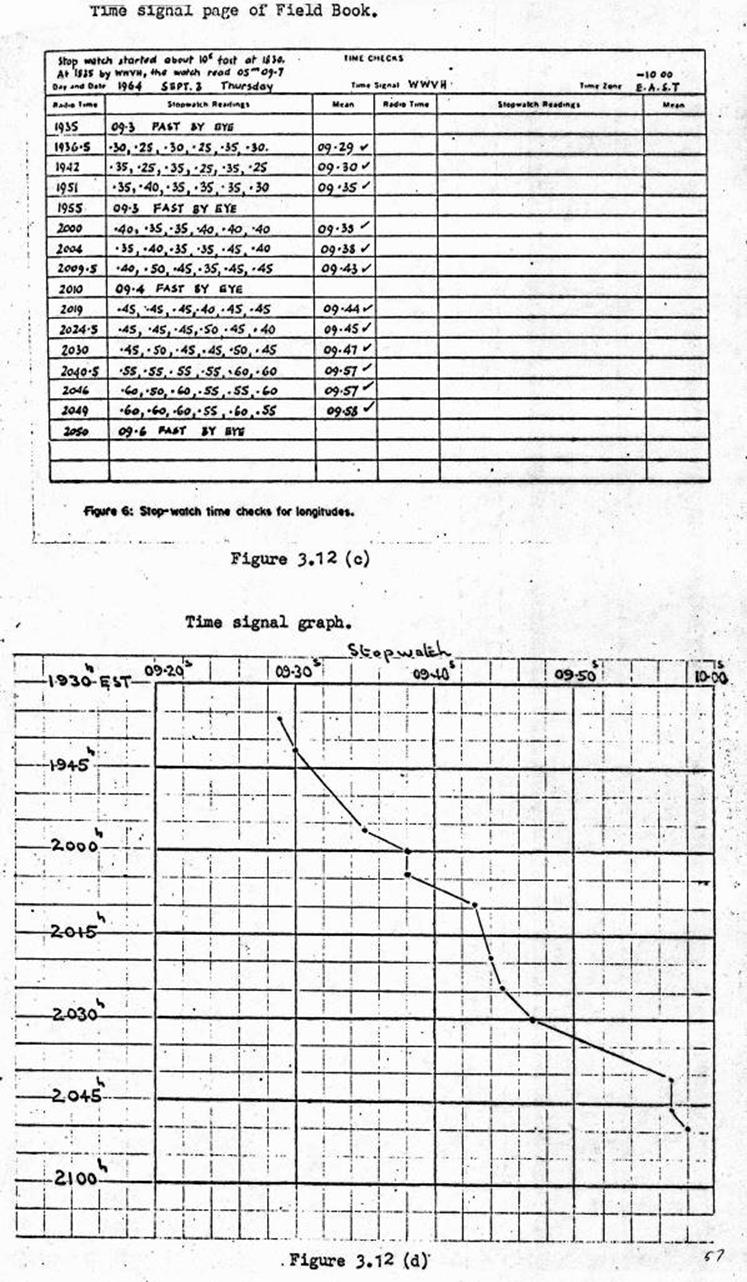
When to take time signals

In the longitude observation using a stopwatch, a fresh time signal is required just before every star; now and again it is permissible to omit one of these signals when stars follow in close succession, however never book more than two stars without taking time signals. If there is a long interval of about 10 or more minutes between stars, a time signal should be taken immediately after the star has been booked and a fresh time signal just prior to the next star.

The "rate" of the stopwatch

This is most likely to be even if the tension on the main spring is kept about the same; therefore make a drill of keeping the watch fully wound – wind it just before taking each time signal. At the conclusion of the observation, graph the time signals at a scale which can easily be read to 0.01 second. Join each point with a straight line. If the correct procedure has been maintained the graph will be reasonably smooth; a "jagged" graph can indicate any of the following and gives warning that some action is required :

i. More practice, or care in beating the stopwatch.

ii. Watch not being kept fully wound, thus tension on the main spring is inconsistent and "rate" suffers.

iii. Watch in poor condition, needs overhaul.

The graph will also show at a glance if too few time signals have been taken, or if they have been inconsistently taken, i.e., a few at close intervals but long gaps between others. Too few time signals combined with a jagged graph would mean the observation must be considered unreliable. See Figure 3.12 (d) for a time signal graph.

It is a good plan, for safety, to have the stopwatch on a loop of string around the neck. Do not let it swing free when not in use but keep in a coat or shirt pocket. Although a stopwatch is robust it must be treated as a delicate instrument where an even "rate" suitable for accurate Longitude observations is required.

Theodolite setup

An observing screen should be used. The tripod should be set on three firmly driven pegs, wooden for preference. Pegs to be driven on an angle in conformity with the slope of the tripod leg.

The tripod should be set so that the theodolite will have two footscrews along the line of the meridian; this can be done accurately enough with a prismatic compass. An essential of this observation is that the alidade bubble must be altered slightly after each timing of the star, by moving the ex-meridian footscrew.

Level the instrument carefully, firstly with the plate bubble then finally with the alidade bubble. The instrument will be used on Face Left to agree with the prediction programme. Set the horizontal circle on the meridian by laying on Sigma Octantis at its calculated true bearing or by turning a true bearing from a distant survey control point, if available.

The Almucantar prediction will be for either 30° or 35° altitude, with 30° being best for the T3. This altitude plus refraction must be set on the vertical circle. With the older model Wild T3 theodolites which have vertical circles that read half the angle, the setting will approximately be 105° 00' 25" or 107° 30' 20" depending whether 30° or 35° predictions are to be used. Clamp the vertical circle firmly, throughout the observations.

The following three points should be kept in mind during this observation.

(i) The essence of the observation is timing a star across a series of 5 hairs, and each time reading the alidade bubble.

(ii) Not one angle is read while laid on each star.

(iii) The only control screws moved are the ex-meridian footscrew to vary the bubble and the horizontal slow motion screw to keep the star close to the vertical wire as it cuts the five horizontal wires.

The observation

Look for a trial star of a fair magnitude to test the predictions, the time set on the prediction watch, the azimuth and altitude setting.

The eyepiece prisms will be required on the theodolite. Stars come into view about two minutes before the predicted time assuming the correct data has been supplied for the electronic computing of the programme. If the star is not sighted fairly close to the predicted time make the following checks in the order listed :

(i) Check that the prediction watch has been set correctly, i.e., 3.94 minutes (3m 56s) per day adjustment may have been applied the wrong way or not applied at all.

(ii) Check that the theodolite has been laid accurately in azimuth.

(iii) Check that the theodolite has been laid on the same Altitude as shown on top of the Almucantar prediction sheet.

If all the above are correct it would appear that an error has been made in the data supplied for the prediction. If this is a gross error it may possibly be rectified if an FK4 star catalogue is available, i.e. locate a well known star which is predicted, observe to the nearest minute its azimuth at the moment it cuts the almucantar circle and record the time to the nearest minute. There is every possibility that if the predicted stars are all corrected by the same difference in bearing and time as indicated by the observation on the known star, the prediction sheet will then be accurate and the observation can go ahead.

If this does not solve the problem it will be necessary to request new prediction sheets.

Assuming that the trial star appeared as predicted, get ready to proceed with the observation :

1) Check and adjust level if necessary.

2) Check that the vertical circle has been set correctly, get booker to record setting on top of field book page.

3) Decide on first star, lay on predicted bearing.

4) Take time signal, record results.

5) Watch for star to come into view; verify its identity by estimating the magnitude, set alidade bubble with the ex-meridian footscrew so that the ends are just a little apart (say between 0.1 & 0.4 of a graduation).

6) With the horizontal slow motion screw the star is positioned so that it will cut the first horizontal wire close to the vertical wire, call to the booker "Star coming in", so that he can concentrate on reading the main watch to the nearest second.

In Australian latitudes the interval between the hairs is about 22 seconds of time; during this interval the observer has to complete the following 4 steps :

1. Call "Up", simultaneously pressing the stop watch button.

2. Read the stopwatch, and when the booker has called back the reading, re-start the second hand.

3. Read the alidade, alter it by touching the ex-meridian footscrew, balancing the error in so doing.

4. Adjust the horizontal slow motion screw to bring the star close to the vertical wire ready for timing it across the next hair.

Proceed with the second, third, fourth and fifth hairs in the same manner. Swing to the azimuth of the next star, making sure that the horizontal slow motion screw is about central in its run.

Take a time signal, return to the theodolite and observe again as outlined for the previous star.

Two points which need further emphasis are :

1. Alidade bubble readings.

The bubble is graduated as shown in Figure 3.12 (a) each division is about 5" to 6" of arc. No attempt is made to bring the ends into exact co-incidence, the readings are estimated to the nearest tenth of a division, and if the reading on the first hair is +0.3, the bubble is altered with the ex-meridian footscrew to read -0.3 for the second hair and so on. If the plus and minus readings over the five hairs are deliberately set so as to almost balance out, any error in the calibrating of the bubble automatically cancels out.

In becoming familiar with his instrument the observer should do two things, i.e. :

1) Move the bubble with the alidade screw and assure himself that the vertical angle is indeed plus or minus of the actual reading when in the positions shown in Figure 3.12 (a).

2) Calibrate the alidade bubble to ascertain the value of the graduations; proceed as follows :

(i) On Face Left lay on some target that can be finely bisected. This is only necessary to prove that the vertical axis is not moved during the course of the calibration.

(ii) To calibrate, move the bubble with the alidade adjusting screw to one end of its run; let it settle.

(iii) Check that the telescope has not been moved off target, read vertical circle and bubble.

(iv) Move bubble about one sixth of its run, let it settle and again take vertical circle and bubble readings.

(v) Repeat until bubble is at the other end of its run. Readings can more advantageously be made more frequently towards the ends of the bubble’s run and less frequently in the middle.

(vi) Check again that the telescope is still on target, and take another series of readings back up the bubble’s run, to the starting point.

(vii) Make a final check that the telescope is still on target.

(viii) Calculation of the value of a division is best done graphically. Firstly convert the T3 readings to seconds of arc remembering that the older model reads only half the angle on the vertical circle and that both models also have the micrometer drum graduated at 60" for a two minute run. Plot a graph of seconds of altitude against bubble divisions. Draw a straight line through the points using a transparent ruler to judge the mean position. Avoid simply joining the two end points, which in effect discards all the other readings. Determine the slope of the line in seconds per division. With some instruments it may be found that separate parallel lines are obtained on the graph, one when the altitude is increasing and the other when it is decreasing - this is due to backlash. When this defect is found, the cure is always to make the last adjustment to the alidade bubble in a clockwise direction, regardless of whether one needs to move the bubble up or down. Few observers do this, and with a new instrument it is not essential, however it is clearly a good habit to get into.

2. Missed Stopwatch readings on any hair

One missed hair does not invalidate that star. If a hair is missed :

(i) In finalizing the field book, the observations for the symmetrical hair must be cancelled. If the first or last hair is missed, use the centre three, if the second or fourth, use hairs one, three and five, if the centre is missed use the other four.

(ii) Observations for the same hairs must be struck out for the other star in the pair.

(iii) Count a pair of stars with missing hairs as half a pair only: if the programme requires eight pairs, they could consist of seven perfect pairs, plus two pairs with missing hairs.

Check the Vertical Setting

After every four pairs, and at the end of the observations, check the vertical circle setting and record it on the top of the page of the field book, thus :

"Vertical circle checked and found to read………………..”

If the setting has changed more than 2", record this and reset the circle to the original value before continuing with the observation. If the error is found while a pair is incomplete, complete that pair before re-setting the circle. Remember that if during the observation of a pair, the vertical circle slow motion screw or the alidade adjusting screw are moved the observation on that pair is ruined.

Booking

As in most astronomical observations, apart from "position lines", the observer relies heavily on his booker. The booker should have a table and chair if possible. If this cannot be managed he must have a large booking board and a rolled up swag to sit on, also a good light which can be shielded so as not to hinder the observer. Paper clips or rubber bands to prevent the field book pages and prediction sheets from becoming unmanageable, are a necessity.

If the booker is experienced, in many ways he will run the observation by selecting the stars, advising the observer when and on which bearing to look for the next star, also advising the time available in which to take a time signal.

The observer will advise "Star sighted" and give estimated magnitude. The, booker will check this with the magnitude of the predicted star and call "Seems OK" or "Large difference in magnitude" as the case may be. Observations on many wrong stars have been prevented by this simple check.

If the magnitude indicated that the correct star was in view the booker carries out the following sequence as the observation on that star progresses :

(i) Writes the page, star number and aspect in the field book.

(ii) Concentrates on the main watch and records in the appropriate "box" the time to the nearest second at the observers call of "Up".

(iii) Enters stopwatch time and bubble reading in the appropriate "box" beneath the main watch time calls these back to the observer.

The above sequence is completed for each of the five hairs; if a hair is missed write that word in the appropriate "box".

On completion of that star the booker calls the next bearing and time available, and so on through the observation, also advises the observer to check the vertical circle after each 4 pairs have been completed. During this observation the booker has no reductions to do; however he should keep alert for gross errors in the stopwatch readings, and mean the 5 bubble readings to ensure they are indeed being "balanced" as mentioned previously and should advise the observer if care is not being taken along these lines.

"Pairs" are numbered as they are completed, not in advance, too often some type of delay prevents a planned observation taking place. With a very experienced booker the best plan is to have all the East stars on the Left hand page and the corresponding West stars on the Right hand page, thus the pairs are on the same line across the double page. However it has been found that a less experienced booker soon enters an East star among the West or vice versa. For this reason it is probably better to enter all stars in chronological order down the page. Always save the prediction sheets and return them with their respective field books. See Figure 3.12 (e), for a field book page.

Observers Personal Equation

This is determined by observing stopwatch longitudes at a station whose longitude has already been determined impersonally. The minimum of observations to give a single reliable calibration would be eight pairs on each of three, or preferably four nights.

As time is not always available for such a programme a good practical solution is to make the normal observation of eight pairs on two nights at the calibration station before the first and after the last of a group of up to 5 new stopwatch longitude stations.

Compilation of Longitude data sheets

The preparation of these for the T3 observation is described in Technical Report No.4. Also there are now available, from the Division's Canberra Office, field books in the form of data sheets for many types of field observation. They incorporate carbon-impregnated paper for the original page, thus the data sheet is available without rewriting and a duplicate copy is left in the field book as a record of the original observations.

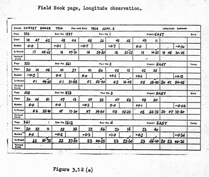
3.13 Latitude observations with the Wild T3 Theodolite – Meridian or Circum-Meridian Altitudes

General

This is the companion observation to the Almucantar Longitude observation. Data sheets for predictions are prepared at the same time as those for Longitude - See Technical Report No. 4 for notes appertaining to the Wild T3.

With that instrument stars within the altitude band 30° to 60° are suitable, and all readings are taken on Face Left.

Much of the data in the notes on the Almucantar observation of Longitude, with the Wild T3 and stopwatchl apply to this observation and will not be repeated, but the main differences in emphasis will be pointed out. These are :

(a) In the Longitude observation, very accurate time and alidade bubble readings are the main factors and no angles are read. In the Latitude observation, almost the reverse applies, very accurate vertical angles combined with alidade bubble readings are the basis of the observation. Time signals are taken in the same manner as described for the Longitude observation but only at the commencement, mid-way and the conclusion of the observation. If cloud causes long delays time signals should then be taken each half hour during this delay. Time signals are graphed at the conclusion of the observation.

(b) Alidade bubble movements in the Longitude observation are made with the ex-meridian footscrew. In the Latitude Observation normal usage of the instrument applies therefore the alidade bubble is moved with the alidade adjusting screw.

Selecting "Pairs"

In contrast to the Longitude observation it is advisable to select pairs in advance of the observation. They are paired North and South within 4° of altitude and 20 minutes of time, trying to find a partner among the many North stars for each of the rarer South stars.

Observations on a single night are acceptable but 8 pairs on each of two nights should be the aim, 12 pairs being the minimum.

Number of Shots per Star

With the wild T3 which has a maximum altitude of about 60°, six shots are required. The maximum time allowed in which to complete these is six minutes, i.e. three minutes each side of upper transit. Note that it is better to obtain a few shots to many stars, than many shots to few stars.

The observation

The setup, laying out of the theodolite on the meridian, time signals etc are as for the Longitude observation except for the slight differences mentioned previously.

If the setting of the horizontal circle and the prediction watch have not already been tested on the Longitude programme, follow the same procedure by checking the transit time and altitude of the first reasonably bright star.

Assuming all is correct proceed as follows :

(i) Set the predicted reading on the vertical circle and swing on to the meridian, North or South as the case may be.

(ii) Find the star, call "Star seen" and verify the magnitude with the booker.

(iii) Estimate how long it will take to get 3 shots before upper transit, move the theodolite horizontally so that the first cut can be taken on the horizontal wire but close to the vertical wire. Set alidade bubble with the alidade bubble adjusting screw just slightly off level, and call "star coming in" to warn booker.

(iv) Call "Up", simultaneously pressing the stopwatch button.

(v) Read stopwatch, bubble and vertical circle. The booker will read these back as they are given. Re-start stopwatch second hand once this has been read back.

(vi) Move alidade bubble fractionally with alidade adjusting screw.

(vii) Again move theodolite horizontally so that the second shot will also be taken close to the vertical wire. Repeat the above sequence until the six shots are taken, a shot every 30 seconds being the aim.

As in the Longitude observation the plus and minus bubble readings should purposely be made to balance out; they should range somewhere between +0.5 and -0.5 over the 6 shots on each star. This system helps to nullify any error in the graduation of the bubble, and also a "sticking" bubble, by keeping the mean altitude almost independent of bubble readings.

The degrees and minutes of altitude need only be read on the first and last shots. After the last shot immediately re-set the horizontal and vertical slow motion screws to the centre of their runs, then set the instrument on the meridian and at the predicted altitude of the next star.

Booking

Most of the general notes regarding booking of the Longitude observation will again apply and the same field book is used.

It is best to book the North stars on the Left hand page and the South stars on the Righthand page, however once again if an inexperienced booker is likely to get them mixed it is better to book them in chronological order down the page. The sequence of operations for the booker is :

(i) Advise the observer the time available, the altitude and aspect of the star.

(ii) Observer will give estimated magnitude; booker will check this with the actual magnitude listed and advise observer if there appears doubt.

(iii) On the observers call "Star coming in", concentrate on the main watch and record time to the nearest second on the call, "Up".

(iv) Read back in turn, stopwatch, bubble and vertical circle readings.

Proceed with steps (iii) and (iv) again until the six shots on that star are completed; enter page, star number, pair number and aspect in the field book. See Figure 3.13 (a) for an example of a field book page.

During gaps in the programme the booker should advise the observer when to look for the next star, when to take time signals etc. He is also responsible for recording temperatures and pressures for Refraction. The thermometer must be hung where it indicates the true external air temperature, the thermometer being read to the nearest degree Celsius and once per pair of stars, unless it is falling rapidly when it should be read once per star.

The pressure should be taken every half hour. If a battery of altimeters is used, readings will later have to be converted to millibars.

Compilation of Latitude data sheets

See notes in Longitude observation.

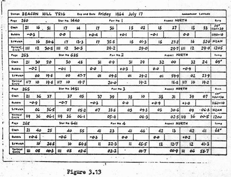
4 Tellurometer MRA-2

4.0.1 Setting up

Set the tripod firmly in the ground using foot pressure on the metal shoes. Level the tripod head by adjusting the tripod legs. In very windy conditions it is wise to take precautions to prevent the instrument from being blown over. The tripod should be securely anchored to the ground by retaining stays tied to the top of the tripod legs. Alternatively rocks can be stacked around the tripod shoes.

Procedure :

(a) Remove from the haversack and place the instrument on the tripod head. Steady it with one hand and secure it loosely with the tripod securing screw. Move the instrument on the ball joint on the head until the point of the plumbob is exactly over the station mark. Tighten the screw until the instrument can just be rotated on the tripod.

(b) Remove the operating-panel cover by unscrewing the wing-headed screw. Also remove the cover of the antenna boss on the side of the instrument by operating the lever and pulling of the cover off.

(c) In order to remove the reflecting dish and the dipole which are securely held inside the operating panel-cover turn the knurled head of the retaining device anticlockwise until the spring-loaded and plunger arm coincides with the long slot. Turn the knurled head up to the limit of the slot then anticlockwise as far as it will go. Disengage the dipole from its spring clip and withdraw the reflecting dish. Protect the dipole while the reflecting dish is being fixed into its position.

(d) Secure the reflecting dish into its operating position on the instrument by inserting the pegs (on rear of the reflector) into the holes provided in the antenna hub releasing the spring-loaded locking lever.

(e) Plug the dipole securely into the sockets.

(f) Using the cable provider connect the instrument to the battery watch carefully that the polarity is correct. The cycle lamp should light up immediately.

(g) Allow 10 minutes for the oven to warm up. The oven should cycle four times before measurements are commenced.

(h) The instrument is now ready to use.

4.1 Description of Tellurometer MRA-2

4.1.1 General

The following is a description of the various assemblies, and controls, switches, meters etc on the operating panel. It also furnishes the operator with sufficient information for the proper operation of the instrument.

The major component assemblies of the instrument are :

(a) the antenna assembly comprising the reflecting dish and dipole.

(b) the instrument case and covers.

(d) the transistorised power supply.

4.1.3 Controls, switches, meters

Brilliance

This control is used to adjust the brilliance of the trace on the cathode ray tube (CRT). The FOCUS control should be used in conjunction with the brilliance control.

Focus

This control is used to adjust the sharpness of the trace on the CRT.

X Shift

This control moves the spot in a horizontal direction across the face of the CRT. It should be adjusted until the spot is a centred within the graticule.

Y Shift

This control moves the spot in a vertical direction across the face of the CRT. It should be adjusted until the spot is centred within the graticule.

Shape

This control is used when the instrument is operating as a MASTER; it adjusts the shape of the display on the face of the CRT. The control should be adjusted until the major axis of the ellipse corresponds with the X axis.

Y Amplitude

This control is used when instrument is operated as a MASTER, in order to adjust the amplitude of the ellipse in the vertical direction until it becomes a circle. After the axes of the ellipse have been bought into coincidence with the X and Y axes of the CRT and the Circle Amplitude control has been used to just the major diameter of the ellipse to be equal to the diameter of the graticule circle, the Y Amplitude control is used to adjust the miner diameter to be the same as the diameter of the graticule circle.

Circle Amplitude

This control is used when instrument is operated as a MASTER, to adjust the circular presentation on the CRT by increasing or decreasing its diameter, until a satisfactory circular trace is obtained.

Check pulse

This switch is used in the Master position to convert the circular presentation on the CRT to a display on the master from the remote station thus the master operator can ensure sufficient pulse is being received from the remote station and if not instruct the remote operator to increase the pulse amplitude.

Graticule lamp

This is used to set the level of illumination necessary on the graticule.

Cavity Tune

This is situated at the top left of the panel and comprises a knob with an integral turns counting dial.

The control is used to adjust the resonance frequency of the cavity by altering the position of double plunger inside the cavity. As the knob is turned clockwise the plunger is moved further into the cavity thus increasing the resonance frequency. When the tuning adjustment is made it is usually necessary to retune the klystron reflector using the reflector tuning control. Tuning of klystron cavity should be undertaken only when the instrument is in the SPEAK position otherwise it is possible to tune into a side band. There are many cavities spaced about 10mc/s apart. The cavity should always be tuned for maximum AVC reading. The Master instrument should always tune to the Remote and should always be 33mc/s lower in frequency. The knob is graduated from 0 to 10 and has a fine scale on which 100 divisions corresponding to one division on the coarse scale.

Speak/Measure switch

This key switch is used to select the “Speak” or “Measure” functions of the instrument. It is also used as a means of signalling when the Master operated wishes the Remote operator to change patterns. When this switch is momentarily flicked from “Measure” to “Speak” the 1kc/s monitoring signals in the remote earphones and on the remote cathode ray disappear, and this is customarily used as an indication to the Remote operator to change to the next pattern.

The Pattern Selector switch

This is located below the Speak/Measure switch. It is used to select first the function MASTER or REMOTE, then the pattern (A, B, C or D), and at the Remote station that type of 1kc/s signal (Forward or Reverse) on the A+ and A- patterns. It has twelve positions as follows :

Master Remote

A A+R, A-R, A-F or A+F

B B

C C

D D

If the selector switches are not synchronised the monitoring signal in earphones and a presentation on the screens of both the Master and Remote stations will disappear.

Pulse amplitude

This is used when instrument is operated as a REMOTE. Adjusting as required by the Master operator in order to increase or decrease the pulse level until the optimum size of the break is obtained on the circular trace.

Reflector tune

This is situated at the bottom left of the panel and is adjusted for peak crystal current which is in effect a measure of the output power from the klystron.

Input supply socket

This is located at the bottom centre of the panel and it should be connected with the cable supplied to the battery.

Power switches

The LT (low tension) On/Off switch is used for switching power to the tube heaters, the klystron heater, and the transistorised power supply. The HT (high tension) On/Off switch, which must be operated not less than half a minute after the LT switch, is used to switching to be +250V and -230V outputs from the power supply.

Fuses

Two fuses are incorporated in the units :

The LT fuse is rated at 10A;

the HT fuse is in the HT line and is rated at 100mA.

Crystal current meter

This is situated to the left of the LT fuse and indicates the current flowing through the crystal mixer in the dipole assembly. The current is adjusted by the Reflector Tune control.

Switched meter

This is situated to the right of the HT fuse, and used in conjunction with the METER selector switch, to monitor the instrument. When the switch is set to REG the meter indications should be between 20 and 80μA. A reading below 20μA indicates a flat battery or faulty power supply. When the switch is in the MOD position the meter should indicate 40μA for the A, B and C patterns and 36μA for the D pattern. When the switch is in the AVC position the meter reading for the short range operations should be about 60μA and for long-range operations about 20μA.

Meter selection switch

This is situated below the HT fuse and is used in conjunction with the Switched Meter above. It has three working positions :

REG : where current through the regulator tubes is measured;

MOD : where the level of the output from the oscillator i.e. the level of modulation is measured;

AVC : where the strength of receiving signals are indicated on the meter.

Panel lamp control

This is situated on the left of the Cavity Tune and it sets the level of the internal illumination of the panel.

Oven cycle lamp

This is situated top centre of the panel. It indicates whether power is being supplied to the crystal oven and lights up when instrument is connected to a battery.

Headset socket

This socket marked PHONE is situated the bottom right of the panel. The headset is plugged into the socket for speech communication.

4.1.4 Pre-operational checking

(a) Switch on the LT switch. After 30 seconds switch on the HT switch.

(b) Set the Meter Selector switch to read REG. A reading of at least 20μA on the Switched Meter indicates a flat battery or faulty power supply.

(c) Set the Speak/Measure switch to Measure and the Meter Selector switch to MOD. Switch the Pattern Selector in turn to A, B, C and D, Master and Remote. In positions A, B and C the reading on the Switched Meter should be 40μA; in position D it should be 36μA.

(d) Rotate the Reflector Tune control for maximum reading on the Crystal Current Meter. A reading of reasonable amplitude signifies that the Klystron is oscillating and the crystal mixer is functioning.

(e) Set the Speak/Measure switch to Speak and check the thermal noise in earphones.

(f) Observe whether there is a spot on the cathode ray tube and check the operation of the X Shift, Y Shift, Focus and Brilliance controls.

(g) Check whether the graticule lamp control varies the level of illumination on the graticule and also whether the panel-lighting control operates satisfactorily.

4.2 Operation under usual conditions

The following general pattern should be followed for all measurements :

(a) Setup the instruments at 2 stations and tune them in.

(b) With the Remote unit, on its initial CAVITY TUNE setting (say ONE) and the Master tuned below it take a complete set of "coarse” readings (A+, A-, B, C, and D). Repeat on cavities THREE and TEN.

(d) On CAVITY TUNE setting TEN, take a set of “fine" readings (A+F, A-F, A-R, A+R). Repeat in half cavity settings down to cavity THREE.

(e) Take a final set of atmospherics. This is also the first set for Remote.

(f) The Remote now becomes the Master, "fine" readings are repeated exactly as in (d).

(g) The final set of atmospherics is taken, followed by three sets of "coarse" readings to complete the measurement. The atmospheric readings are exchanged by the two operators.

4.2.2 Sequential method of measuring with the MRA-2 Tellurometer

Master

Remote

(a)

Rotate the Cavity Tune knob for about half a rotation on each side of the previously decided starting point. If the Remote is not yet switched on to SPEAK only a small deflection of the needle will be seen. In this case, keep on turning the control through the above tuning range until the meter deflection becomes large; then carefully tune for maximum deflection, adjusting the CAVITY TUNE and REFLECTOR TUNE controls.

Set the CAVITY TUNE knob to the previously decided starting point (say 5.0). A large increase in the reading on the SWITCHED METER indicates that the Master instrument is in contact with the Remote.

(b)

Adjust the direction of the instrument for maximum AVC reading.

Adjust the direction of the instrument for maximum AVC reading. Listen for any instructions from the Master.

(c)

Record the REG reading.

(d)

Instruct the Remote operator to switch to MEASURE. Switch to MEASURE and MASTER A positions. Using the CIRCLE AMP control, set the circle to a reasonable diameter.

When instructed, switch to MEASURE and Remote A+F positions.

(e)

Adjust the brightness, focusing, position and shape of the circle. Re-adjust the diameter of the circle. Make a final adjustment of the REFLECTOR TUNE for a suitable break in the circle. (Failure to obtain any break or a break of suitable width must be treated as an instrumental fault.)

Check the presentation, adjustment. (BRILLIANCE, FOCUS, X SHIFT, and Y SHIFT.

(f)

Switch to SPEAK and instruct the Remote operator that "coarse" readings will now be taken. Set the Speak/Measure switch to MEASURE. Read the angular position (between 0 and 100) of the leading edge of the break in the circular trace. (If the circle is traversed in a clockwise direction the first edge of the break that is encountered is the leading edge). Record this reading and the A+ reading. Momentarily flick the Speak/Measure switch to indicate to the Remote that he must change patterns. Take another reading of the position of the leading edge of the break. Record this as the A- reading.

When instructed that "coarse" readings are to be taken switch to MEASURE and either listen to the tone signal, in the earphones or watch the pulse display on the cathode ray tube. When they disappear momentarily switch to the A-F position.

(g)

Switch the pattern selector to MASTER B. When the circular trace reappears, take a reading and record it as the B reading.

When the display and tone disappear, switch the pattern selector to REMOTE B.

(h)

Repeat (g) for the MASTER C and D positions.

Repeat (g) for the REMOTE C and D positions.

(i)

Switch to CAVITY TUNE 3. Tune to the Remote as motioned in (a). Take a set of coarse readings as described in (f) to (h).

Switch to CAVITY TUNE 3. When contact is made with the Master, switch to MEASURE and proceed with coarse readings as described in (f) to (h).

(j)

Switch to CAVITY TUNE 10. Tune to the Remote as motioned in (a). Take a set of coarse readings as described in (f) to (h).

Switch to CAVITY TUNE 10. When contact is made with the Master, switch to MEASURE and proceed with coarse readings as described in (f) to (h).

(k)

Switch to SPEAK and instruct the Remote operator to take a set of atmospheric readings. Calculate the vapour pressure, and compare with the Remote to see they come within the allowable limits.

When instructed take a set of atmospheric readings. Calculate the vapour pressure, and compare with the Remote to see they come within the allowable limits.

(l)

Inform the Remote operator that

Fine readings will now be taken.
Allow the Remote operator sufficient time to return to his instrument; then with the REFLECTOR TUNE control adjust for maximum AVC reading. Switch to MEASURE. Take a reading on the CRT graticule and record it as the A+F reading. Flick the Speak/Measure switch and record the next reading as the A-F. Repeat for A-R and A+R.

When instructed by the Master operator that Fine readings will now be taken adjust the REFLECTOR TUNE control for peak crystal current. When instructed switch to MEASURE. When the tone or the display disappear momentarily switch to the A-F position. Repeat for A-R and A+R. Note this order must be adhered to unless changed prior to measuring by the Master operator.

(m)

Switch to SPEAK get Remote AVC reading. Instruct Remote operator to change frequency.

Retune the instrument to its new setting below that of the Remote.

Take a further set of 4 "fine" readings.

Switch to SPEAK report Remote AVC reading, change to the frequency instructed by the Master operator, switch to A+F and repeat step (l).

(n)

Repeat step (m) through the tuning range.

(o)

Take a set of atmospheric readings, compare vapour pressure as before.

(p)

This completes one half of the measurement. The Remote operator now becomes the Master operator and the measurement proceeds.

The Remote operator now changes to Master operator, and the measurement proceeds.

The sequence for this second half of the measurement is in reverse of the first half, the order being :

(i) Fine readings.

(ii) Atmospherics.

(iii) Coarse readings.

Atmospherics are now exchanged, also any data about eccentric or station marks. The instrument can now be packed away. First switch off the HT, then the LT, disconnect the battery, headset, dipole and reflecting dish.

4.2.3 Operation over land

Although in principle, any line over which it is possible to transmit and receive signals, can be measured by the Tellurometer system, circumstances may be such that a choice of sites for the instrument can be made. This applies particularly to surveying in country where beacons either do not exist, or need not be used. As operation of the instrument at sites with suitable properties may improve the accuracy and ease of measurement, some attention should be paid to site selection.

Two factors influence the choice of a line for good working reception of signals and ground reflection.

In the first place, the line should be free from obstruction, and the plane of the radio beam (22° wide), should not be obstructed for the first 30 metres. This latter point can be ensured by raising the instrument about 2 metres, if the ground is level; or by selecting a site where the ground falls gradually away from the station for at least 30 metres. The terrain should be free from obstructions such as trees or buildings in a cone of about 10° on each side of the line. If it is impossible to select a site with this last requirement it is essential that the trees do not move during the measuring period. In other words wait for still weather conditions.

In the second place a line should be selected so that the ground reflection effects are negligible. Since this is not usually possible, the next best course is to select sites that result in at least one full cycle of swing.

If the ground is well wooded or otherwise broken up, the indirect ray can be scattered, and not reflected. Even in this event the power of the indirect ray which reaches the receiver may not be negligibly small. To prevent the resulting errors it is best to adopt the second procedure above, i.e., to select a line that has good ground reflection properties and results in at least one cycle of swing.

Such a line has a ground clearance of about 70 metres over a distance of 32km, 45 metres over a distance of 16km, and so on. Since more than one cycle of swing is desirable, sites with clearances at the middle point of over 70 metres for 32km lines, over 45m for 16km lines and over 30m for 8km lines and so on, should be selected.

4.2.4 Operation over water

Certain conditions of a water surface, such as a very choppy sea, can cause scattering of the indirect ray, in a similar manner to rough ground; but, in general, the conditions are similar to those of flat, bare ground.

An additional effect from an over water path, is a regular or irregular change in the length of the indirect ray due to a vertical rise and fall of the surface caused by "swell". This rise and fall results in a changing of the relative phase of the direct and indirect rays, in the same way as a change of carrier frequency does. Thus, if the carrier frequency were kept constant, the readings would nevertheless swing about a mean value; in principle, it would be sufficient to average this swing, instead of obtaining a swing by frequency diversity. In practise, however, an operator cannot be certain that a full swing has been developed, and the method of frequency variation must be carried out.

Since "swell" can introduce errors even though frequency is employed, sites should be selected where possible so that the ground obscures the water surface from the instrument thus there will be no reflection from the water. Sometimes this can be made possible by lowering the instrument.

4.2.5 Atmospheric effects

The final limiting factor in obtaining maximum accuracy, at medium and long ranges, is the effect of atmospheric conditions. The procedure set out for taking atmospheric readings, can be regarded as being adequate under most conditions. This procedure assumes that the atmospheric conditions along the line are constant or vary uniformly. If either condition does not exist, an error in measurement can result.

Since there is no way of determining the atmospheric conditions along the line, the best procedure is to carry out measurements during periods of certain weather conditions.

Fine, dry, sunny weather, which induces vertical air currents are ideal. A fair breeze, blowing along the line, is to be preferred to any other type of wind. Night measurements tend to be less accurate than day measurements.

In damp climates measurements on cooler days will be more accurate than those on warmer days when the vapour pressure may be higher. In coastal areas anomalies may be experienced due to variations in vapour pressure along the line; however, in general the vapour pressure is constant over large areas and changes only slowly with time.

4.3 Field computation of Tellurometer measurements

For the reduction of vapour pressure, dry and wet bulb temperatures are required, also the barometric pressure. Tables have been made up so that these can be calculated using Centigrade readings for temperature, and millibar readings for pressure. See (h) below. NOTE : The tables in these notes have been constructed with Excel and final values differ from the original tables above 30 degrees by up to 0.04 due to evaluation of power term.

Taking the readings :

(a) The dry and wet bulb reading of the psychrometer should be taken with the instrument in the shade and at the height of the instrument. The psychrometer should be held well away from the observer’s body and in a position where the air-vent is pointing into the wind. The observer should watch the mercury throughout the observation. The mercury sometimes tends to oscillate, but readings should not be made until the thermometers have reached their minimum values. It will take 3 or more minutes for this to happen.

(b) The thermometers are calibrated and the chart showing the index corrections for the temperature ranges should be kept in the box containing the psychrometer.

(c) The time of observation is recorded to the nearest minute and the Master operator enters his wet and dry bulb readings, in their appropriate column in the field book. The index corrections are then applied, and the final values entered.

(d) The results are checked with the Remote operator to see that the vapour pressure, at each end of the line, agrees within the required limits before "fine" readings are proceeded with.

(e) The wick on the wet bulb should be kept clean, and replaced when dirty. Only clean water should be used. Be sure no water gets on the dry bulb.

In the Bendix model, care should be taken to ensure that the batteries are in good condition.

(f) The barometer should be read immediately after the dry and wet bulb temperatures have been read. The readings should be recorded in the appropriate places in the field book, index corrections applied, and the final adopted values shown.

(g) Barometer comparisons should be carried out at regular intervals throughout the course of the survey. The mechanism barometers are compared against a standard mercury barometer at a Department of Civil Aviation Meteorological Office or other Meteorological Station.

(h) Figures 4.3.1(a) & (b) show Tables "A" & "B". These are' necessary to calculate the Vapour Pressure from the atmospheric readings. A set of these tables must be carries with each instrument to enable the calculated vapour pressure at each end of the line to be compared before and after each measurement. This is to ensure that they agree within the limits specified for the particular task in hand. Figure 4.3.2 shows these calculations on the appropriate field book page.

TABLE A		Δe = 0.00066(1+(0.00115t'))p
WET
BULB	Millibars
Celcius	820	830	840	850	860	870	880	890	900	910	920	930
0	0.541	0.548	0.554	0.561	0.568	0.574	0.581	0.587	0.594	0.601	0.607	0.614
5	0.544	0.551	0.558	0.564	0.571	0.578	0.584	0.591	0.597	0.604	0.611	0.617
10	0.547	0.554	0.561	0.567	0.574	0.581	0.587	0.594	0.601	0.608	0.614	0.621
15	0.551	0.557	0.564	0.571	0.577	0.584	0.591	0.598	0.604	0.611	0.618	0.624
20	0.554	0.560	0.567	0.574	0.581	0.587	0.594	0.601	0.608	0.614	0.621	0.628

25	0.557	0.564	0.570	0.577	0.584	0.591	0.597	0.604	0.611	0.618	0.625	0.631
30	0.560	0.567	0.574	0.580	0.587	0.594	0.601	0.608	0.614	0.621	0.628	0.635
35	0.563	0.570	0.577	0.584	0.590	0.597	0.604	0.611	0.618	0.625	0.632	0.639
40	0.566	0.573	0.580	0.587	0.594	0.601	0.608	0.614	0.621	0.628	0.635	0.642
45	0.569	0.576	0.583	0.590	0.597	0.604	0.611	0.618	0.625	0.632	0.639	0.646
	Millibars
	940	950	960	970	980	990	1000	1010	1020	1030	1040	1050
0	0.620	0.627	0.634	0.640	0.647	0.653	0.660	0.667	0.673	0.680	0.686	0.693
5	0.624	0.631	0.637	0.644	0.651	0.657	0.664	0.670	0.677	0.684	0.690	0.697
10	0.628	0.634	0.641	0.648	0.654	0.661	0.668	0.674	0.681	0.688	0.694	0.701
15	0.631	0.638	0.645	0.651	0.658	0.665	0.671	0.678	0.685	0.692	0.698	0.705
20	0.635	0.641	0.648	0.655	0.662	0.668	0.675	0.682	0.689	0.695	0.702	0.709

25	0.638	0.645	0.652	0.659	0.665	0.672	0.679	0.686	0.693	0.699	0.706	0.713
30	0.642	0.649	0.655	0.662	0.669	0.676	0.683	0.690	0.696	0.703	0.710	0.717
35	0.645	0.652	0.659	0.666	0.673	0.680	0.687	0.693	0.700	0.707	0.714	0.721
40	0.649	0.656	0.663	0.670	0.677	0.683	0.690	0.697	0.704	0.711	0.718	0.725
45	0.653	0.659	0.666	0.673	0.680	0.687	0.694	0.701	0.708	0.715	0.722	0.729
FORMULAE	:	e = e' - (t - t') Δe		and		Δe = 0.00066 (1+(0.00115 t')) p
				and		e' = 6.107* (10^ ((7.5* t') / (237.3+ t')))

where	:	T	is the	dry bulb temperature °C
		t'	is the	wet bulb temperature °C
		e	is the	Vapour pressure (millibars)
		e’	is the	Vapour pressure at saturation (millibars) (Table B)
		p	is the	barometric pressure millibars
		Δe	from	Table A

To find Vapour Pressure e :					Example :
					Pressure		1010	Millibars
					Dry bulb		26.1	°C
					Wet bulb		24.4	°C
					Depression		1.7	(Dry - Wet)
(a)	Extract value from Table B
	for wet bulb temperature				From Table B - wet bulb value extract :						30.56

(b)	Extract constant from				From Table A - wet bulb & pressure values extract :						0.686
	Table A and multiply by						multiply by wet bulb depression				1.7
	wet bulb depression.						subtract from Table B value				1.166
	Subtract from Table B value							e	millibars	=	29.39

Figure 4.3.1(a) : Table "A"

TABLE B					Vapour pressure at saturation - e'
WET
BULB	0	0.1	0.2	0.3	0.4	0.5	0.6	0.7	0.8	0.9
0	6.107	6.152	6.196	6.242	6.287	6.333	6.379	6.425	6.472	6.519
1	6.566	6.614	6.661	6.710	6.758	6.807	6.856	6.905	6.955	7.005
2	7.055	7.106	7.157	7.208	7.260	7.312	7.364	7.417	7.469	7.523
3	7.576	7.630	7.685	7.739	7.794	7.849	7.905	7.961	8.017	8.074
4	8.131	8.189	8.246	8.304	8.363	8.422	8.481	8.541	8.601	8.661
5	8.722	8.783	8.844	8.906	8.968	9.031	9.094	9.157	9.221	9.285
6	9.349	9.414	9.480	9.545	9.612	9.678	9.745	9.812	9.880	9.948
7	10.017	10.086	10.155	10.225	10.295	10.366	10.437	10.509	10.580	10.653
8	10.726	10.799	10.873	10.947	11.021	11.096	11.172	11.248	11.324	11.401
9	11.478	11.556	11.634	11.713	11.792	11.872	11.952	12.033	12.114	12.195
10	12.277	12.360	12.443	12.526	12.610	12.695	12.780	12.865	12.951	13.038

11	13.125	13.212	13.300	13.389	13.478	13.567	13.657	13.748	13.839	13.931
12	14.023	14.116	14.209	14.303	14.397	14.492	14.587	14.683	14.780	14.877
13	14.975	15.073	15.172	15.271	15.371	15.472	15.573	15.674	15.777	15.879
14	15.983	16.087	16.192	16.297	16.403	16.509	16.616	16.724	16.832	16.941
15	17.050	17.160	17.271	17.382	17.494	17.607	17.720	17.834	17.948	18.063
16	18.179	18.296	18.413	18.530	18.649	18.768	18.888	19.008	19.129	19.251
17	19.373	19.496	19.620	19.745	19.870	19.996	20.122	20.250	20.378	20.506
18	20.636	20.766	20.897	21.028	21.160	21.293	21.427	21.562	21.697	21.833
19	21.969	22.107	22.245	22.384	22.524	22.664	22.805	22.947	23.090	23.234
20	23.378	23.523	23.669	23.816	23.963	24.111	24.260	24.410	24.561	24.712

21	24.865	25.018	25.172	25.327	25.482	25.639	25.796	25.954	26.113	26.273
22	26.434	26.595	26.758	26.921	27.085	27.250	27.416	27.583	27.750	27.919
23	28.088	28.259	28.430	28.602	28.775	28.949	29.124	29.300	29.476	29.654
24	29.833	30.012	30.193	30.374	30.556	30.740	30.924	31.109	31.295	31.483
25	31.671	31.860	32.050	32.241	32.433	32.626	32.820	33.015	33.212	33.409
26	33.607	33.806	34.006	34.207	34.410	34.613	34.817	35.023	35.229	35.437
27	35.645	35.855	36.066	36.278	36.490	36.704	36.919	37.136	37.353	37.571
28	37.791	38.011	38.233	38.456	38.680	38.905	39.131	39.358	39.587	39.817
29	40.048	40.280	40.513	40.747	40.983	41.219	41.457	41.696	41.937	42.178
30	42.421	42.665	42.910	43.156	43.404	43.653	43.903	44.154	44.407	44.660

31	44.915	45.172	45.429	45.688	45.948	46.210	46.473	46.737	47.002	47.269
32	47.537	47.806	48.076	48.348	48.622	48.896	49.172	49.449	49.728	50.008
33	50.289	50.572	50.856	51.142	51.429	51.717	52.007	52.298	52.590	52.884
34	53.180	53.477	53.775	54.075	54.376	54.678	54.982	55.288	55.595	55.903
35	56.213	56.525	56.838	57.152	57.468	57.785	58.104	58.425	58.747	59.070
36	59.395	59.722	60.050	60.380	60.711	61.044	61.379	61.715	62.053	62.392
37	62.733	63.075	63.419	63.765	64.112	64.461	64.812	65.164	65.518	65.874
38	66.231	66.590	66.951	67.313	67.677	68.043	68.410	68.779	69.150	69.523
39	69.897	70.273	70.651	71.031	71.412	71.795	72.180	72.567	72.955	73.345
40	73.738	74.131	74.527	74.925	75.324	75.725	76.128	76.533	76.940	77.349
	This table was constructed with Excel and differs from the original,
	above 30 degrees by 0.04, due to evaluation of power term

Figure 4.3.1(b) : Table "B"

The formulae form which these tables are calculated are :

e = e’ – (t-t’)*Δe and Δe = 0.000 66(1+0.00115*t’)p

e’ = 6.107 *10a where a = (7.5t’)/(237.3+t’)

where :

e = Vapour pressure (millibars)

t = dry bulb temperature °C

t’ = wet bulb temperature °C

p = barometric pressure millibars

e’ = Vapour pressure at saturation (millibars) (Table B)

Δe = Table A

Example :

Wet bulb 24.4°C, Dry 26.1°C, Pressure 1010.0mbar

Δe = 0.000 66(1+0.00115*24.4)*1010.0 = 0.6853

0.686 from Table A

a = (7.5*24.4)/(237.3+24.4) = 0.6993

e’ = 6.107x10^0.6993 = 30.556

30.556 from Table B

e = 30.553 – (26.1-24.4)*0.686 = 29.391

29.390 using Tables

4.3.2 Atmospheric readings required for the computation

These have been taken simultaneously, at each end of the line :

(a) Immediately before the first "fine" readings were commenced.

(b) At the Conclusion of these "fine" readings.

Dry bulb, Barometric Pressure and Vapour Pressure for (a) and (b) at both stations, are meaned and used in calculating the first measurement.

Dry bulb, Barometric Pressure and Vapour Pressure for (b) and (c) at both stations, are meaned and used in calculating the second measurement.

See 4.3.2 for an example of atmospheric readings and calculation.

4.3.3 Explanation of the “coarse” figure

Coarse patterns are :

A-B 10 kc/s pattern 50,000 ft. (15,240 metres)

A-C 100 kc/s pattern 5,000 ft. ( 1,524 metres)

A-D 1000 kc/s pattern 500 ft. ( 152.4 metres)

A alone 10 mc/s pattern 50 ft. ( 15.24 metres)

For lines longer than 50,000ft (15,240 metres) the first figure must be provided by a rough knowledge of the length of the line :

KILOMETRES			MILES
0 to 15	first figure	0	0 to 10	first figure	0
15 to 30		1	10 to 20		1
30 to 45		2	20 to 30		2
45 to 60		3	30 to 40		3
60 to 75		4	40 to 50		4
75 to 90		5	50 to 60		5

Example of a set of coarse readings, rough distance between 15 & 30km

A+ 16 A+ 16 A+ 16 A+ 16 (add 100, if necessary)

B 09 C 42 D 75 A- 84

07 74 41 2) 32

16 (should be close to A+)

"Coarse” figure : 1 0 7 4 16 (first figure is 1 as distance 15-30km)

Example of a set of coarse readings, rough distance between 30 & 45km

A+ 06 A+ 06 A+ 06 A+ 06 (add 100, if necessary.)

B 75 C 80 D 36 A- 92

31 26 70 2) 14

07 (should be close to A+)

"Coarse” figure : 2 3 2 7 07 (first figure is 2 as distance 30-45km)

Ambiguous discrepancies in the difference readings

Assume that the following readings are obtained :

A+ 16 A+ 16 A+ 16 A+ 16

B 09 C 42 D 78 A- 80

07 74 38 2) 36

A= 18

Considering the A-D figure, it is seen that the 8 of the 33 does not readily check with the 1 of the 18. On the other hand, considering the A-C figure, the 4 of the 74 checks with the 3 of the 38; thus it may leave some doubt whether the coarse figures are 07318 or 07418. However, since only 3 needs to be added to 38 to give 41, a value of which the 1 checks with the 1 of the 13, it can be seen the 33 should be 41, the discrepancy being due possibly to a alight error in the instrument, or in the reading of the trace. Then the 4 of the 74 checks with the 4 of the 41, and the 1 of the 41 with the 1 of the 18. Thus the coarse figure is 07418.

“Bracketing” method to resolve ambiguities

In the measurement under discussion the difference readings are :

A-B 07, A-C 74, A-D 38 and A 18. Proceed as follows;

(i) Write down the A-D and A figures on the one line with a bracket in the space between the, thus : 38 [ 18

(ii) Enter in the centre of the bracket a figure which consists of the tenths digit of the A-D value, and the tenths digit of the A value :

38 [31 18

(iii) Bracket the figure so obtained with values 10 above and 10 below, thus :

38 [31 18

The value in the bracket that is closest to the observed value is the true difference reading, i.e., of the three, 41 is closest to 38. Therefore the A-D coarse digit is 4.

Where it is necessary to carry out this method on the A-C, and A-B values as well, always treat the A-D reading first, then repeat the others, thus :

A+ 16 A+ 16 A+ 16 A+ 16

B 09 C 38 D 18 A- 80

07 78 98 2) 36

A= 18

01√

98 [91 18

80√ Step 1

78 [70 01

18 Step 2

07 [08√ 80

Step 3

Step 1 : The correct A-D value is 01, therefore use the "0" (tenths digit) in Step 2.

Step 2 : The correct A-C value is 80, therefore use the "8" (tenths digit) in Step 3.

Step 3 : The correct A-B value is 08.

The coarse figure therefore is 08018, which is not readily apparent from the difference readings.

Unresolvable difference readings

Consider the following set of readings :

A+ 16 A+ 16 A+ 16 A+ 16

B 11 C 37 D 74 A- 76

05 79 42 2) 40

A= 20

The 2 of the 42 (A-D value) checks with the 2 of the 20 (a value). Using the method of “bracketing” on the A-C value the following is obtained :

79 [74 18

However, as 79 is midway between 74 and 84, the A-C value can either be 74 or 84, and the coarse reading 07420 or 08420.

Provided that there is not too large a difference between the A+ and A values, the A value can be substituted for the A+ value, in evaluating the, difference readings, thus:-

A+ 20 A+ 20 A+ 20 A+ 16

B 11 C 37 D 74 A- 76

09 83 46 2) 40

A= 20

This gives a coarse figure of 08420 which should be correct. However to accept these figures would not be good surveying practise, therefore the coarse figures should be taken again, preferably with a different instrument.

The cause of ambiguities in the Coarse readings

Assuming the trace has been properly centralised with the graticule, and the operator has not made a consistent mistake in all 3 sets of coarse readings the cause of an ambiguity in the readings is that the A+ and A- readings do not approximately total 100. (The A- reading is an A+ reading taken in a counter-clockwise direction).

Therefore, if the A+ and A- readings usually total in the vicinity of 92, or 108, or worse, difficulty probably will be found in resolving coarse readings. If this is the case the instrument should be returned for adjustment.

Care with Coarse readings

A-B crystal gives the value of the distance up to 99,999mμ/s, thus an error of 1 in the resolving of this coarse figure will give an error of 10,000mμ/s (5000ft or 1524metres). This is easily traceable from a map.

A-C crystal gives the value of the distance up to 9,999mμ/s, thus an error of 1 in resolving this coarse figure will give an error of 1,000mμ/s (500ft or 152metres).

A-D crystal gives the value of the distance up to 999mμ/s, thus an error of 1 in resolving this coarse figure, will give an error of 100mμ/s (50ft or 15metres).

An error of 500 feet or less could not be ascertained from the 1:250,000 map which will normally be the most accurate map available for scaling the check distance. Therefore the correct resolving of the coarse figures is essential.

4.3.4 Simple explanation of the Tellurometer measurement

The following is included to enable operators to more readily comprehend the broad basis of the Tellurometer measurement.

The instrument measures the time taken for a radio wave to travel from one Station (the Master) to the other (the Remote) and back to the first. The unit of time used is the millimicrosecond (mμs), which is a thousandth of a millionth of a second.

Suppose the transit time is 10,000 milli-microseconds, i.e., ten millionths of a second.

As the wave travels about 186,000 miles in one second, in ten millionths of a second it travels :

(186,000 / 1,000,000) * 10 = 1.86 miles.

As this is the double path length the single path distance is 0.93 miles.

Metric equivalent :

The wave travels about 299,792km in one second, in ten millionths of a second it travels :

(299,792 / 1,000,000) * 10 = 2.998km.

As this is the double path length the single path distance is 1.499km.

As the wave travels along the path it meets resistance from the atmosphere. A correction is applied for this and the resultant answer is the distance between the stations.

To eliminate any errors from a single reading (which could be caused by ground reflection), a series of 15 "fine" readings are taken on successive carrier frequencies.

4.3.5 Booking and field calculation of a Tellurometer measurement

Figure 4.3.2 shows the atmospheric observation page, vapour pressure calculations, and the mean of the readings from both stations, as required to calculate the measurement. The necessary tables to do these calculations should always be carried with each instrument.

Figure 4.3.5.(a) shows the coarse figure and its reduction. Three sets of coarse readings are taken from each station. A graph of the fine readings and the description of the quality of the trace are also shown on this page.

Figure 4.3.5.(b) shows a set of 15 "fine" readings. The booker receives these from the operator, in the order : A+, A-, A-R, A+R. He can usually calculate the differences and fill in these two columns, as the readings are being taken. The mean differences and the "fine" readings can be quickly calculated at the conclusion of the measurement. REG and A MOD readings and the commencement and finishing times of the measurement, are noted.

The AVC readings at both stations, for each "fine" reading are noted as the reading is taken. This may be required later on, to give an idea of the quality of the signal on each cavity.

The 15 cavities are meaned. As a check, all columns can be totalled and cross-checked, as shown, to also provide the mean of the 15 cavities.

The calculation page of the field book is shown in Figure 4.3.5.(c). This shows the calculation being done in the following steps :

(i) Transit time entered and halved.

(ii) Half Transit time x 299 7925 gives measured distance, in metres.

(iii) Atmospheric correction is worked out, using this formula :

n-1 = [ {77.601*(P+E) / (273+t)} * 10-6] and E = (4744 e) /(273+t)

Referring again to Figure 4:3.5(c) we find the following atmospheric observations are to be used :

Dry bulb temperature t = 15.4°C

Vapour pressure e = 8.218 millibars

Baro. pressure P = 972.19 millibars

Compute E first :

273 + t (15.4) = 288.4 so 4744 *e (8.218) /288.4 =135.18 = E

P+E = 972.19 +135.18 =1107.37 so 77.601 *1107.37 /288.4 =297.964

Thus the atmospheric correction for 1,000,000 metres is 297.964; for 100,000 metres it would be 29.796 metres and for 10,000m it would be 2.9796 metres.

The correction for the above measurement of 14,135.240m is :

297.964 X 10-6 x 14,135.240m = 4.211 metres

Eccentric corrections

It is best to draw a diagram roughly to scale even though very small. This gives the approximate correction, but more importantly ensures that the correct sign is used.

The calculation is :

Distance eccentric to station mark x Cos angle station mark to Distant Station

Where the angle is 0° to 90° and 270° to 360°; correction is minus.

Where angle is 90° to 270° correction is plus.

Slope correction

This is rarely needed in the field. The difference height between the stations is necessary. Calculate with the formula provided :

Slope correction = Diff Height^2 / 2 * Slope distance

Sea Level correction

Also rarely needed in the field. Mean height of stations necessary. Calculate with the formula provided :

Sea Level correction = (Mean height * slope distance) / (R + mean height) where R = 6,378,160m

Chord to Arc correction

Also rarely needed in the field. Tables (4.3.5(g)) are available and should be carried if precise field computations are to be made. Can be calculated with the formula provided :

Chord to Arc correction = Slope distance^3 / (43 * {6,378,160}2)

4.4 Fault finding procedure

When repairs are being undertaken in the field, certain precautions should be observed in order to ensure the safety of the personnel and prevent mistakes that can cause a major break-down of the equipment.

The antenna dipole always should be handled carefully. When the back cover of the instrument is off and inspections are being made, the power supply should be switched off. Accidental contact with the klystron circuit when the power is on can result in a bad electrical shock.

The fault finding procedure as set out, should be applied in locating faults in the instrument, which has largely been designed to be self-monitoring. Using the indications on the instrument, all but the most obscure sources of failure should be apparent without the use of separate equipment, except perhaps, a general-purpose, high-impedance, DC meter.

Certain types of component failure are to be expected from time to time in any electrical equipment. As a reasonable safeguard, the instruments are supplied with spare parts kits for use in the field. These spare parts should be sufficient for 1000 hours operation.

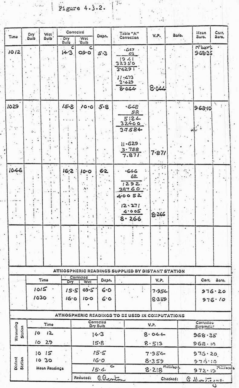
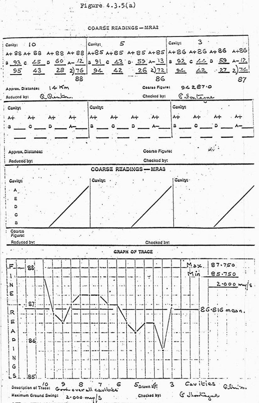
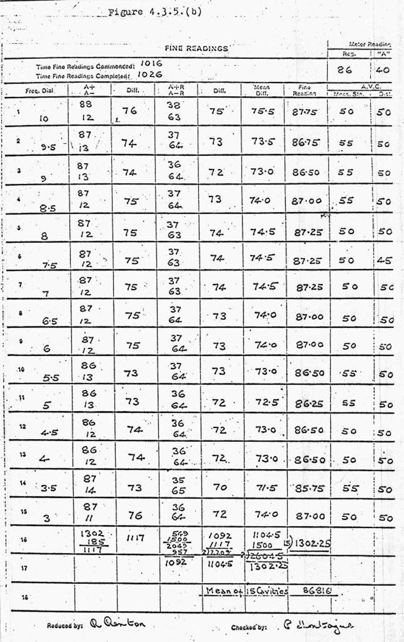
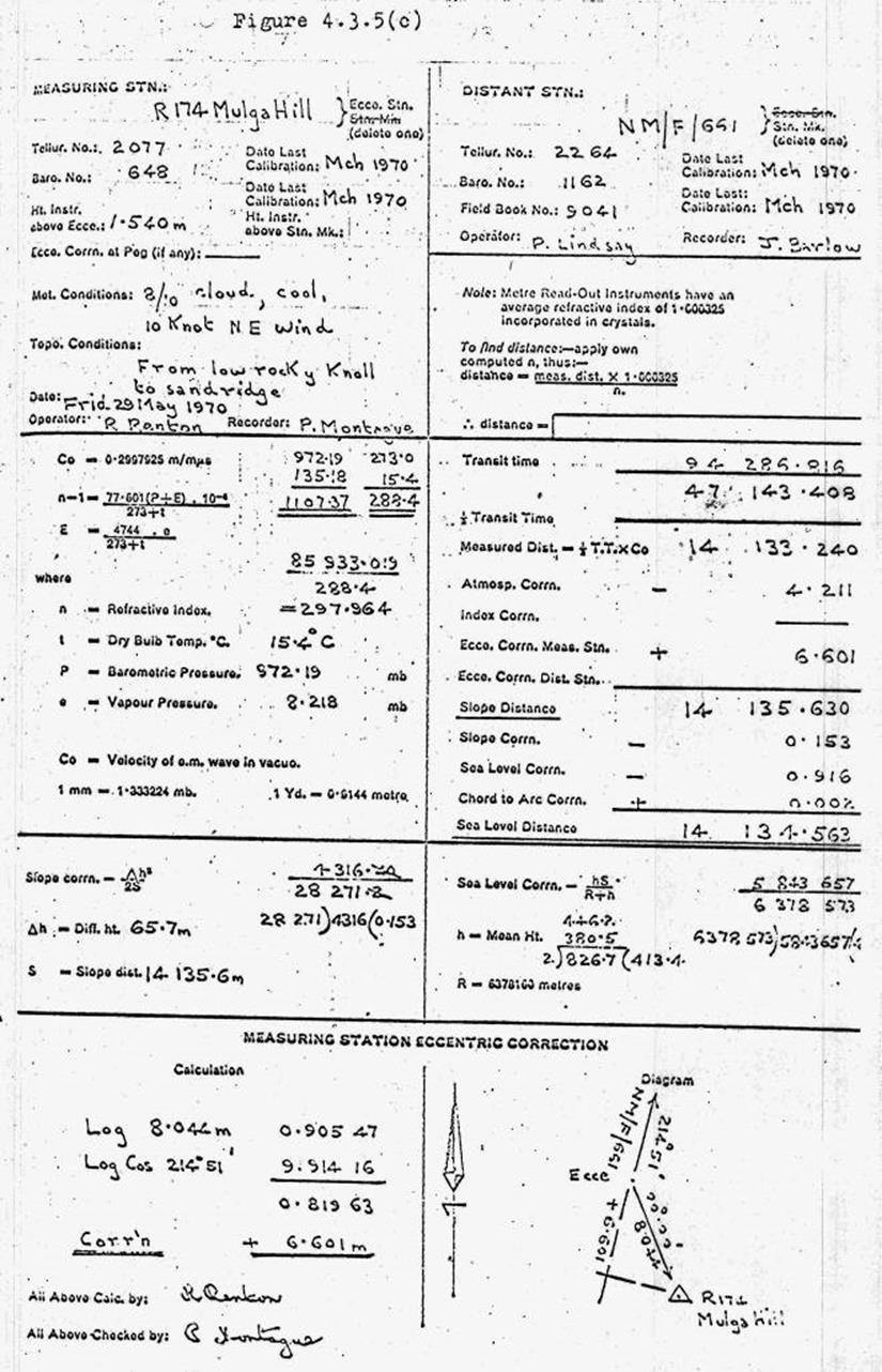
CHORD TO ARC CORRECTION TABLES
Chord to Arc correction = Slope distance³ / (43 * {6 378 160}²)
All values in metres (slope distances are x1000 metres)

Distance	Correction	Distance	Correction	Distance	Correction	Distance	Correction
10	0.001	41	0.039	71	0.205	101	0.589
11	0.001	42	0.042	72	0.213	102	0.607
12	0.001	43	0.045	73	0.222	103	0.625
13	0.001	44	0.049	74	0.232	104	0.643
14	0.002	45	0.052	75	0.241	105	0.662
15	0.002	46	0.056	76	0.251	106	0.681
16	0.002	47	0.059	77	0.261	107	0.700
17	0.003	48	0.063	78	0.271	108	0.720
18	0.003	49	0.067	79	0.282	109	0.740
19	0.004	50	0.071	80	0.293	110	0.761
20	0.005	51	0.076	81	0.304	111	0.782
21	0.005	52	0.080	82	0.315	112	0.803
22	0.006	53	0.085	83	0.327	113	0.825
23	0.007	54	0.090	84	0.339	114	0.847
24	0.008	55	0.095	85	0.351	115	0.869
25	0.009	56	0.100	86	0.364	116	0.892
26	0.010	57	0.106	87	0.376	117	0.916
27	0.011	58	0.112	88	0.390	118	0.939
28	0.013	59	0.117	89	0.403	119	0.963
29	0.014	60	0.123	90	0.417	120	0.988
30	0.015	61	0.130	91	0.431	121	1.013
31	0.017	62	0.136	92	0.445	122	1.038
32	0.019	63	0.143	93	0.460	123	1.064
33	0.021	64	0.150	94	0.475	124	1.090
34	0.022	65	0.157	95	0.490	125	1.117
35	0.025	66	0.164	96	0.506	126	1.144
36	0.027	67	0.172	97	0.522	127	1.171
37	0.029	68	0.180	98	0.538	128	1.199
38	0.031	69	0.188	99	0.555	129	1.227
39	0.034	70	0.196	100	0.572	130	1.256
40	0.037

4.4.1 Faults common to the Master and Remote Functions

Complete failure of the instrument

If the Oven Cycle lamp is not burning, check the connections to the battery. Check the LT fuse. Check that the battery is charged.

No noise in the earphone, but a spot on the CRT.

Check the HT fuse and replace, if necessary.

No crystal current

Replace the crystal mixer in the end of the dipole assembly.

Check whether the klystron heater is glowing. If it is not, replace the klystron. To do this, first switch off the instrument and disconnect it from the battery. Turn the Cavity Tune control completely anti-clockwise, and remove the back cover of the instrument. Disconnect the leads to the klystron. Slacken both retaining rings of the cavity (that at the base end of the klystron, first) and slide the klystron out of the cavity, and towards the antenna boss. Reverse the procedure when inserting a new klystron.

No AVC reading, no speech communication, no pattern on the CRT

Check whether the heaters of all the IF tubes are glowing.

Replace any defective tube.

Low AVC reading, no speech communication, no pattern on the CRT

Check that the antenna is directed towards the other instrument.

No speech communication but instrument operates on measure

Check that the headset plug is fully inserted in its socket.

Normal AVC reading, normal speech, 1kc/s note in earphone but no pattern on the CRT

Check brilliance control.

Check tubes V301 and V302 by replacement.

Replace CRT.

No pattern on the CRT, no 1kc/s note in earphone, but speech normal

Check that the pattern selector is set to the correct position.

Check that the pattern selector of the second instrument is set to the correct pattern.

Set the Meter switch to MOD and check all the levels. If these levels are zero on all patterns, check V202 and V203 by replacement

Horizontal deflection but no vertical deflection on the CRT

Replace V303.

4.4.2 Faults peculiar to the Master Function

No circle, but speech and 1kc/s note are normal

Adjust the Circle Amplitude control in case the diameter of the circle is larger than the CRT screen.

Increase the Brilliance.

Follow checks listed in 4.4.1(h)

No phase indicating break, but circle, 1kc/s note and speech are satisfactory

Press Check Pulse button and view the CRT.

Adjust the Reflector Tune control for maximum height of the pulse trace.

If the maximum pulse height is 6mm (¼") or more, release the Check Pulse button and view the circular trace. If no break is evident reduce the brilliance to the minimum usable level.

If the maximum pulse height is less than 6mm (¼"), check whether the pulse is indicated on the Remote CRT. If it is, increase the Remote pulse amplitude.

If no pulse trace is obtained, replace V201. If the fault persists, check the Remote, according to 4.4.3.(b).

Circle cannot be centred on the CRT

In the higher magnetic latitudes this fault is probably caused by the strong vertical magnetic intensity. If that is the case, an adjustment to the CRT divider chain must be made in an approved Maintenance, Depot before the instrument can be satisfactorily used. All MkII instruments have had this adjustment incorporated.

4.4.3 Faults peculiar to the Remote Function

No horizontal trace but a vertical trace on the CRT

Check tubes V301 and V302, by replacement.

No pulse display on the CRT

Check tube V201, by replacement.

Check tube V303, by replacement.

4.4.4 Anomalous CRT displays

In certain circumstances the trace on the Master CRT may not have the ideal form.

Mistuning of the klystron cavity produces a triangular display. Tuning should always be carried out when the Speak/Measure switch is set to Speak.

An elliptical pattern on one position of the pattern selector switch indicates that particular pattern frequency needs to re-adjusted in a Maintenance Depot. Such a pattern should not be read.

A distorted circle can be caused by too large a pulse. If the reducing of the Remote pulse amplitude does not cure the fault, the instrument should be returned to a Maintenance Depot. However, an instrument with this fault can be used, for no reading error is introduced by the distortion.

Multiple circles are caused by either fluorescent lights, when the instruments are being checked indoors, or engine ignition if the instrument is connected to the battery of a car whose engine is left running. This display also can be caused by a defective power pack.

Multiple concentric circles (i.e., circles that change diameter without altering the angular reading of the break) may be caused either by reflections from a moving object or by heat refraction on lines with low ground clearance over the entire distance. Such a display may be read without error.

Rotation of the break backwards and forwards round part of the circle may be caused by reflected signals from a moving object,that are stronger than the direct signal.

"Snow" is caused by scattering of the signal by moving leaves in the line of sight.

A "noisy" or "grassy" display is usually caused by weak signals. It can also be caused by a defective power pack. Provided that the break is evident, its position can be read without error. Reducing the CRT brilliance to the lowest usable level helps to clear the break.

4.4.5 Trouble shooting

The charts (Figures 4.4.5(a) and (b) outline the course to be taken in the event of a failure of the equipment during operation in the field. It must be stressed that any fault that is not given here must be rectified in a Maintenance Depot.

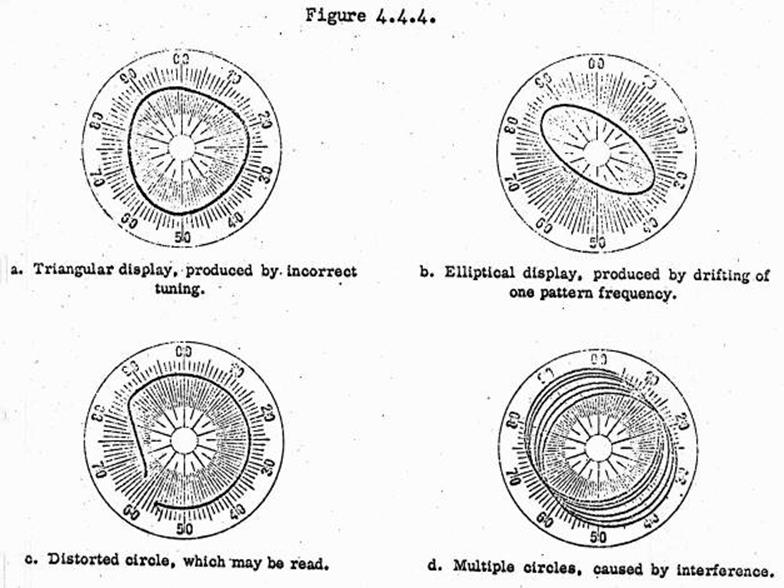
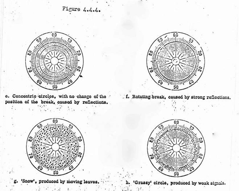
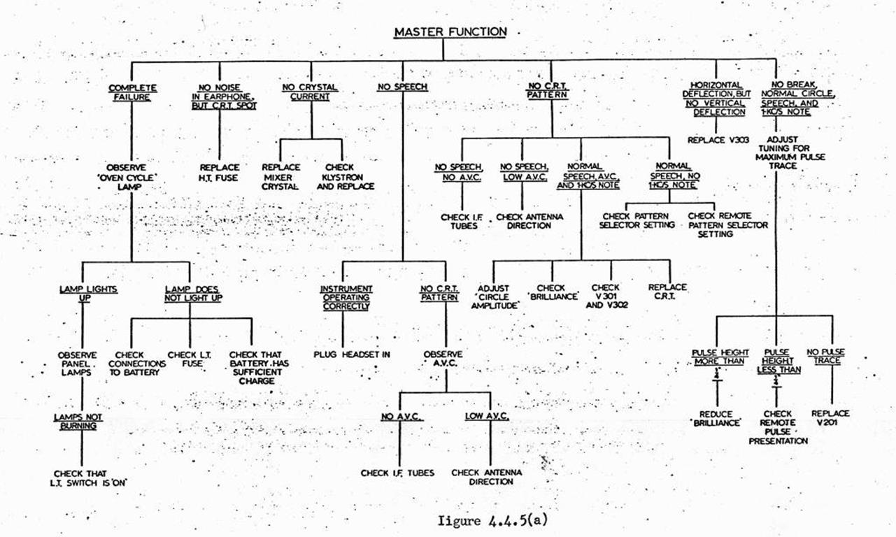
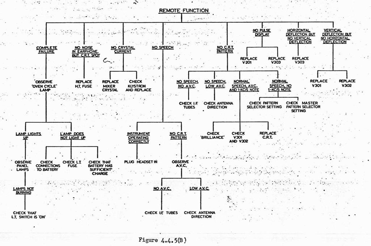
4.5 Tellurometer MRA-3, Dial read-out Unit – 10m/Hz Instrument

4.5.1 General Principles

With a pattern frequency of 10m/Hz (previously 10mc/s), one complete rotation of the Phase Control and the Phase Indicator (0-100 divisions on the main scale) represents a change of 100 nano-seconds (previously milli-microseconds) in the transit time over the double path. Each division therefore, represents one nano-second and is equivalent to a distance of just under 6 inches (15cm), a complete rotation of phase being approximately equivalent to 50 feet (17m approx).

The 10m/Hz pattern, or A pattern, thus indicates the final digits in the transit time in nano-seconds, the preceding figures whole number of rotations of the A pattern being unknown. These are resolved by providing four further patterns. The pattern frequencies are :

A Pattern 10.000m/Hz

B Pattern 9.999m/Hz

C Pattern 9.990m/Hz

D Pattern 9.900m/Hz

E Pattern 9.000m/Hz

The Remote frequencies differ from these by 1k/Hz.

The differences between the readings from the A pattern and the B, C, D and E, patterns, respectively give phase readings relative difference frequency of the modulations, and thus coarse patterns are derived, from which the preceding figures are determined. These coarse patterns, together with the A pattern, are shown in the following table.

A – B	1 k/Hz pattern	500 000 ft
A – C	10 k/Hz	50 000 ft
A – D	100 k/Hz	5 000 ft
A - E .	1 m/Hz	500 ft
A alone	10 m/Hz	50 ft

See 4.5.3 for the conversion of transit time to distance.

4.5.2 Simplified theory of measurement

The following is a simplified theory of measurement is included in these notes to enable operators to readily comprehend the broad basis of the Tellurometer system. The five difference patterns can be represented by five wheels, namely the A, B, C, D, and E wheels. Imagine that the circumference of each wheel is marked by ten equally spaced divisions, and all the wheels rotate together along a given path. Consider each wheel in turn.

A Wheel

As this wheel is rotated along the path, the circumference divisions of the wheel indicate the distance traversed. When a complete revolution is made by the wheel, ten units of distance are indicated by the divisions. When the wheel is further rotated, the indications of distance continue, but the observer cannot determine the preceding number of completed revolutions, and is therefore unable to evaluate the total distance. In order to do this it is necessary to have a second wheel - the E wheel.

E Wheel

The circumference of the E wheel is ten times greater than that of the A wheel, therefore the circumferential length of each of its ten divisions is equal to the whole circumferential length of the A wheel. When the A wheel has made one revolution, the E wheel will have traversed the path of one division. Consequently; when the A wheel has rotated through ten revolutions, the E wheel will have moved through only one revolution, and will thus measure the length of the path in terms of 100 A division units.

When the E and A wheels are further rotated along the path, the observer will again be unable to determine the preceding number of complete E wheel revolutions, and so it is necessary to add three further wheels to complete the system.

D, C and B Wheels

The D wheel has a circumference that is ten times greater than that of the E wheel; therefore the same principle applies for determining the E wheel revolutions by observing the D wheel division marks, as described for the E and A wheels.

Two further wheels complete the system. These are the C having a circumference ten times greater than that of the D wheel, and the B, with a circumference ten times greater than that of the C wheel.

Thus by observing the division marks on all five wheels the distance along the path can be determined in terms of A wheel divisions. The A wheel measures the units of length, and the E, D, C, and B wheels measure the tens, hundreds, thousands, and tens of thousands of A units, respectively.

4.5.3 Conversion of Time to Distance

Suppose the transit time is 10 000 nano-seconds, i.e. ten millionths of a second. As the wave travels approximately 299,792km per second, in ten millionths of a second it travels :

(299 792 / 1 000 000) * 10 = 2.998 Km which is double path distance.

Thus the single path distance is 1.499 Km. In other words, distance = ½Velocity x transit time.

If the velocity is considered constant, the wheels can be calibrated directly to distance units. However, the velocity varies slightly with the atmospheric refractive index, in the following manner, therefore for results of the highest accuracy corrections to the velocity must be made from a knowledge of the refractive index.

Thus, actual velocity = (299792 / refractive index) km/s.

4.5.4 Zero error

The coarse readings, (A, B, C, D, and E) being difference readings, are free from errors produced by constant phase shift in the instrument.

An error can arise from contamination of the measuring signal derived in the Master unit by the measuring signal returned from the Remote, and vice versa. To eliminate this error, a simple reversal of phase by 180° is provided by the forward/reverse switch. This is the equivalent of taking face left and face right readings on a theodolite.

4.5.5 The Control Panel — Description and location of components

Fuse

Rated at 5A and situated at lower left of panel, protects instrument against serious damage in event of component failure, or reversing of battery polarity.

Oven lamp

Indicates when crystal oven heater is on. Periodic switching indicates that the oven is being maintained at correct temperature.

Panel lamps

Used to illuminate the panel for night time operation.

Open vents lamp

Red lamp, is situated at the tog left of the panel; it lights if the internal temperature exceeds 50°C. When lamp lights, the operator should pull open the two vents at the top and bottom of the radome cover; these should be left open until the instrument is switched off.

Power switch

Five position switch, is situated towards the lower left hand corner of the control panel, and can be set to permit operation from either an internal or an external battery. "Warm Up" brings into use the (12V) supply to the crystal oven and the LT power pack. "On" brings into use the HT power pack.

Monitor switch

Six position switch, on lower right hand side of the panel; is used for monitoring purposes. By means of this switch, the battery volt (Batt), mixer crystal current (Xtal), received signal strength (AGC) tuning level (Tune), and modulation levels of the oscillator crystal (Mod), can be indicated on the Monitor meter, which is situated at the top left of the panel. When the switch is in the Speak or Measure positions, it is used to select the speech measure functions of the instrument.

Master/Remote function switch

Multi-position switch, which is situated at the left hand side of the panel; is used for selecting the pattern frequency and Master/Remote function during the measuring process.

AGC switch

This two position switch allows a voltage to be applied to the klystron for automatically controlling the carrier frequency relative to the other instrument.

Forward/Reverse switch

Two position switch used for selecting forward and reverse signals in the elimination of instrumental errors.

Headset connector socket

Marked Mic, and accepts headset plug.

Battery connector socket

Marked Batt, and connects 12 volt external battery.

Volume control

Marked Vol, and is used for adjusting level of sound in the headset.

Panel lighting control

Marked Dim, and is used for adjusting the illumination of the panel.

Cavity tune control

In conjunction with the indicator above, it is used for selecting the cavity frequency. The indicator will vary between 000 and 200.

Monitor meter

Situated in the top left hand corner of the panel. This meter is used in conjunction with the Monitor switch as previously explained.

Read-out units

These are plug in units and are situated on the upper right hand side of the control panel. The one in general use within the Division is the Dial Read-Out unit in nano-seconds. This is the unit to which these operational notes apply.

4.5.6 Dial Readout Unit (nanoseconds)

Description

The Phase-control Knob is centred on a circular main scale which is graduated in 100 equal divisions; every tenth division from zero upwards is numbered in a clockwise direction around the face of the dial. A fixed pointer with vernier scale is mounted centrally, on top of this main scale. The main scale can be rotated against the pointer by turning the Phase-control Knob. The vernier scale indicates the fraction (in tenths of a division), with respect to any whole division on the main scale. There is a "white dot" on the Phase-control Knob.

A light friction drive is provided between the Phase- control and the main scale permitting the scale to be held stationary while the Phase-control is rotated. When a locking device, which is located on upper left quarter of the disc, is engaged with a notch in the rim of the disc, the main scale is held in the position indicating zero on the vernier.

The Null meter is mounted above the Phase-control, panel illumination lamps are provided, one on each side of the meter.

Figure 4.5.(a) shows the operating panel of the MRA-3 Tellurometer with this dial read-out unit.

Operation

These notes outline the general operation of the dial read-out unit, the method of fitting this operation into an actual measurement is laid down in the section, "Sequential method of operating the MRA3 Tellurometer."

At a given Cavity Tune setting, a null position is obtained. By having zero on the main scale locked against the pointer, the null position is then used as a reference against which subsequent readings are taken, thus eliminating the need for numerical subtraction of one reading from the other.

Step 1 Obtaining the null position

Bring the locking device into contact with the rim of the main disc by sliding the button towards the centre of the disc.

Rotate the Phase-control knob, either clockwise or anti-clockwise until the locking device engages with the notch in the rim of the main scale disc, and the disc is held stationary. The main scale is then set with zero against the vernier pointer.

Continue to rotate the Phase-control knob until the needle of the Null meter is in the centre of its scale, (the Null position.)

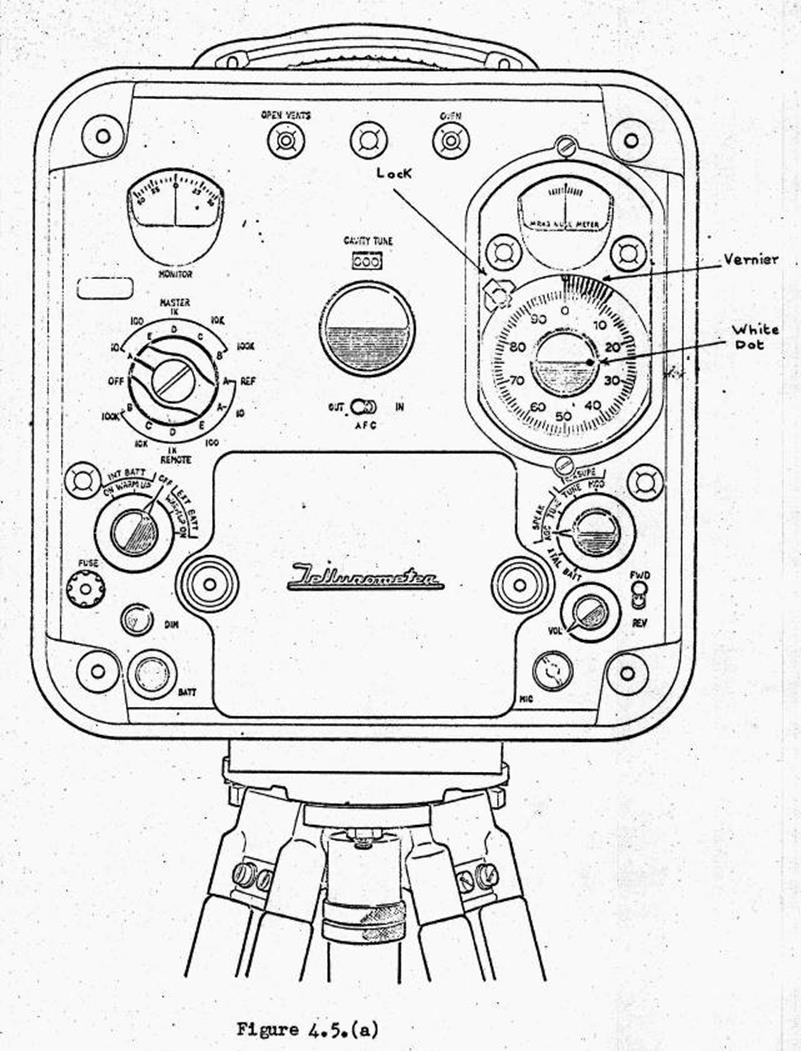
Note : It is possible to obtain two null positions 180°,(or 50 scale divisions) apart. Only one of these positions is correct. When a clockwise rotation of the Phase-control knob causes the meter needle to move clockwise; (or an anti-clockwise rotation causes the needle to move anti-clockwise), the Null position is the correct one. When a rotation of the Phase-control knob causes the needle to move in the opposite sense, the position in the incorrect one. The correct condition for a Null reading is therefore obtained by a continued rotation of the Phase-control knob in clockwise, (or an anti-clockwise) direction, until the movements of the Phase-control knob and the meter needle are in the same sense.

Now book the reading of the position of the "white dot". This reading is the approximate “A” reading, and is a check against taking readings 50 cycles, i.e, 180° in error.

Step 2 Obtaining a reading

Disengage the main scale by sliding the button of the locking device away from the disc. The main scale will now rotate with the Phase-control knob.

Rotate this knob until a Null is obtained on the Null meter.

The correct Null position is only obtained when the needle of the Null meter moves up to the Null position in the same sense as the direction of rotation of the Phase-control knob, irrespective of whether that knob has been rotated through a complete revolution or not.

When the needle of the Null meter is in its Null position read the main scale division which is opposite the pointer, then the decimal part of the division against the vernier. Record the value read, in the appropriate column of the field book.

Figures 4.5.(b), (c), (d) and (e) show the pages of a fie book and include the field computation of the measurement.

4.5.7 Making contact, preliminary arrangements

It should be noted that this instrument is much more directional than the MRA-2 Tellurometer; therefore arrangements for making contact should include :

(i) Ascertaining as accurately as possible the bearing of the distant station.

(ii) Time, make contact.

(iii) Which operator is to be Master.

(iv) On which cavity, contact is to be made; (normally cavity 100).

(v) Procedure for a radio call in the event of failure to make contact by Tellurometer.

4.5.8 Sequential method of operating the MRA-3 Tellurometer

Checking instruments - Master & Remote, identical procedure

(i) Set power switch to EXT BATT/WARM UP.

(ii) Five or ten minutes later move switch to ON.

(iii) Set MONITOR switch to BATT; Monitor meter should read between 20 a 25 if battery is sufficiently charged.

(iv) Set MONITOR switch to MEASURE/MOD; rotate MASTER/REMOTE switch to patterns. Meter should indicate between 40 and 45 for all patterns except MASTER E and REMOTE E where it should be between 30 & 35.

(v) Set MONITOR switch to SPEAKGC.

The sequence, which from hereon differs between Master & Remote is as follows :

MASTER

REMOTE

Making contact

AFC switch to IN

MASTER/REMOTE switch to A MONITOR switch to SPEAKGC

CAVITY TUNE to 065. Rotate control towards 100, watching for maximum deflection of MONITOR meter. This normally occurs about 15 below REMOTE i.e., about 35 in this case.

Make speech contact.

AFC switch to OUT

MASTER/REMOTE switch to A+ REF MONITOR switch to SPEAKGC

CAVITY TUNE to 100. Listen & watch MONITOR meter; when its reading moves from a low to high value, contact has been made by Master. Speech can now heard.

Instruct REMOTE to DF his instrument to improve signal strength.

When instructed, DF to obtain maximum deflection on MONITOR meter. Check plumbob is still over station mark. Advise MASTER when completed.

DF Master instrument to obtain maximum deflection on MONITOR meter. Check plumbob is still over station mark.

Stand by

Set MONITOR switch to SPEAK/TUNE and adjust CAVITY TUNE control for a zero, (+ 5) , reading on the MONITOR meter; check that equal and opposite rotations of this control result in equal and opposite deflections of the meter needle.

Stand by

Check for periodic switching of the Oven lamp.

Taking "coarse" readings

Instruct REMOTE to switch to MEASURE/ TUNE. Set MONITOR switch to MEASURE/TUNE check MASTER/REMOTE switch is on MASTER A. Adjust CAVITY TUNE control for a zero, (±5), reading on the MONITOR meter.

When instructed, set MONITOR switch to MEASURE/TUNE, check MASTER/REMOTE switch is on REMOTE A+ REF, and FORWARD/REVERSE switch on FWD, (switch is normally spring-loaded to stay on FWD on most instruments).

Obtain NULL point. (See 4.5.6. Step 1) and record position of "white dot".

Stand by

Switch, momentarily, to MASTER E and then back to MASTER A, to signal to REMOTE.

When 1k/Hz tone in headset is interrupted, switch to REMOTE A‑

Obtain reading, (see 4.5.6. Step 2.) Call to booker who records and calls back.

Stand by

Switch to MASTER E

When 1 k/Hz tone in headset is interrupted, switch to REMOTE E

Obtain and book E reading

Stand by

Switch to D, C, & B, in turn, obtaining and booking readings.

Switch to D, C, & B, in turn, on interrupted tone signal.

Switch to MASTER A and check first reading.

Switch to REMOTE A- to check first reading.

MONITOR switch to SPEAK/TUNE.

MONITOR switch to SPEAK/TUNE when Master speaks.

Instructs REMOTE to cavity for next set of "coarse" readings. (Usually Cavity 170, then 40.)

MONITOR switch to SPEAKGC; rotate CAVITY TUNE towards 170, watching for maximum deflection of monitor meter.

Make speech contact.

MASTER/REMOTE switch to A+ REF, MONITOR switch to SPEAKGC, CAVITY TUNE to 170. Listen & watch MONITOR meter; when its reading increases from a low to high value contact has been made and speech can be heard.

Set MONITOR switch to SPEAK/TUNE and adjust CAVITY TUNE for a zero,(±5), reading on the MONITOR meter; check that equal and opposite rotations of this control result in equal and opposite deflections of the meter.

Stand by

Master and Remote now follow previously outlined steps for taking "coarse” readings until the "coarse" readings on Cavity 170, and the other necessary cavity are completed. The Master then arranges for simultaneous atmospheric readings.

Taking "Fine" readings

(Assuming last "coarse" reading was on cavity 40, fine readings will start with that cavity.)

Instruct REMOTE that "Fine" readings will be taken. Switch to MASTER A & MEASURE /TUNE, readjust CAVITY TUNE for a zero, (±5) reading on the MONITOR meter.

When instructed, switch to REMOTE A+ REF and MEASURE/TUNE. FORWARD/ REVERSE switch on FWD.

Obtain NULL point (Step 1, 4.5.6. except unnecessary to record position of white dot.)

Stand by

Interrupt tone to signal to REMOTE by momentarily switching to MASTER E and back to MASTER. A.

On hearing interrupted tone, switch to REMOTE A-

Obtain readings (Step 2, 4.5.6).

Call reading to booker who records and calls back.

Stand by

Signal to REMOTE

On hearing signal, switch to REMOTE A+ REF, and hold FORWARD/REVERSE switch down on REV.

Obtain NULL point, as previous.

Stand by

Signal to REMOTE

On signal, switch to REMOTE A- keeping FORWARD/REVERSE switch down on REV.

Obtain reading, as previous.

Stand by

Switch to SPEAKGC and instruct (or signal) REMOTE to change to next cavity.

On instructions (or signal), let FORWARD/REVERSE switch spring back to FWD; switch to REMOTE A+ REF. Set MONITOR SWITCH to SPEAKGC. CAVITY TUNE to next setting (in this case, 50).

Rotate CAVITY TUNE through increasing numbers until a peak reading is obtained on the MONITOR meter. This occurs normally at about 15 below the REMOTE, i.e., about 35 in this case. Set MONITOR SWITCH to SPEAK/TUNE and adjust CAVITY TUNE to obtain a zero, (±5), reading on the MONITOR meter.

Stand by

Instruct REMOTE to switch to MEASURE/TUNE. Set MONITOR switch to MEASURE/TUNE and readjust CAVITY TUNE for a zero, (±5), reading on the MONITOR meter.

Change to MEASURE/TUNE.

Master and Remote now follow previously outlined steps for taking "Fine" readings, until they are completed on this cavity and the other necessary cavities. Simultaneous atmospheric readings are then arranged by the Master.

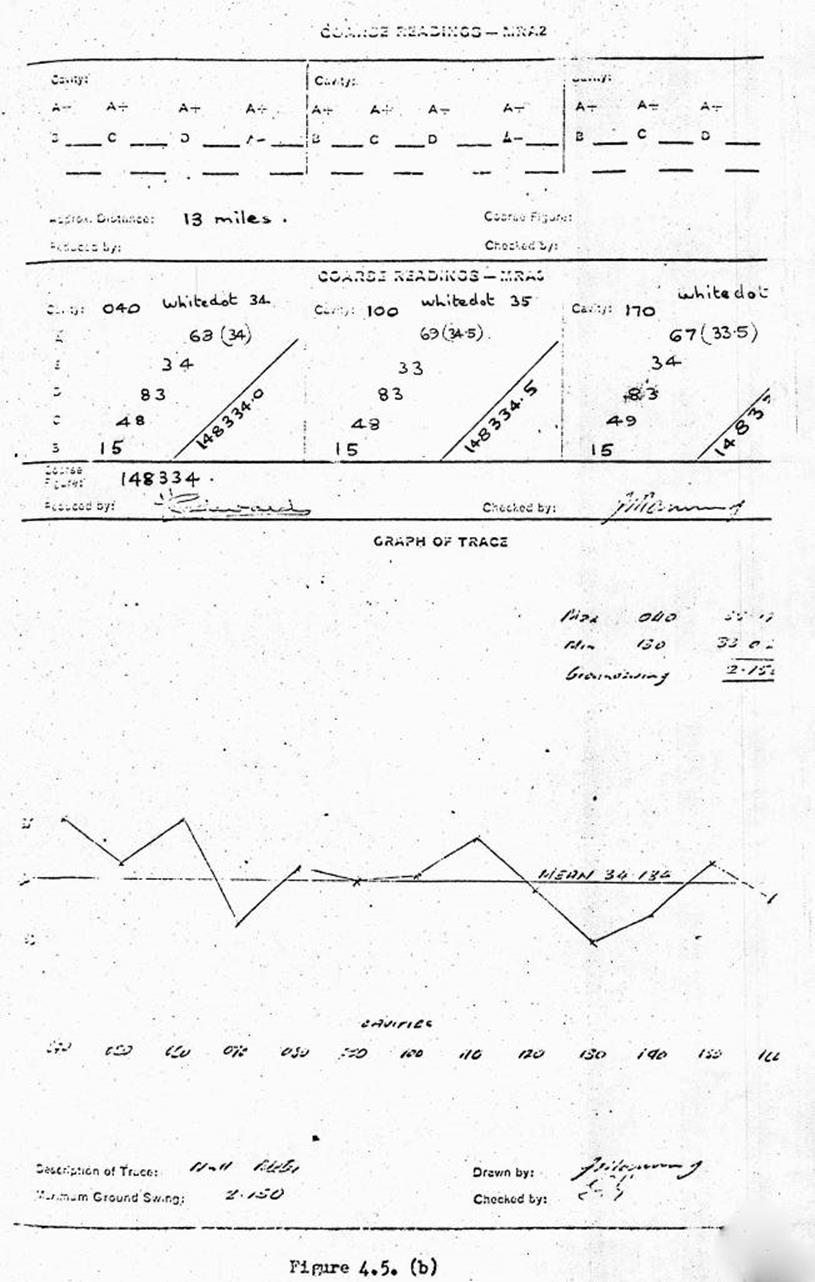
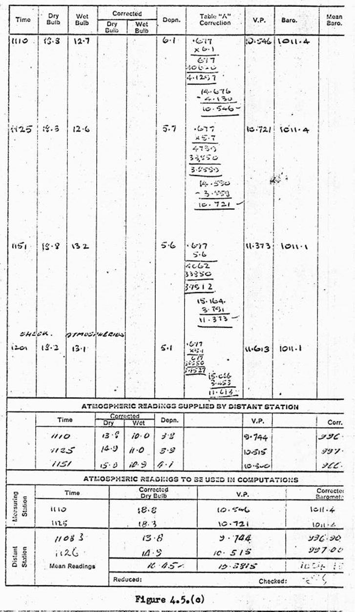
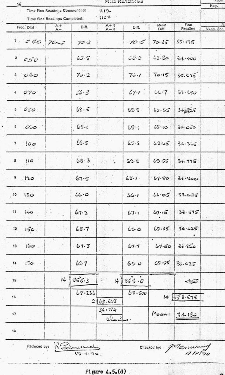
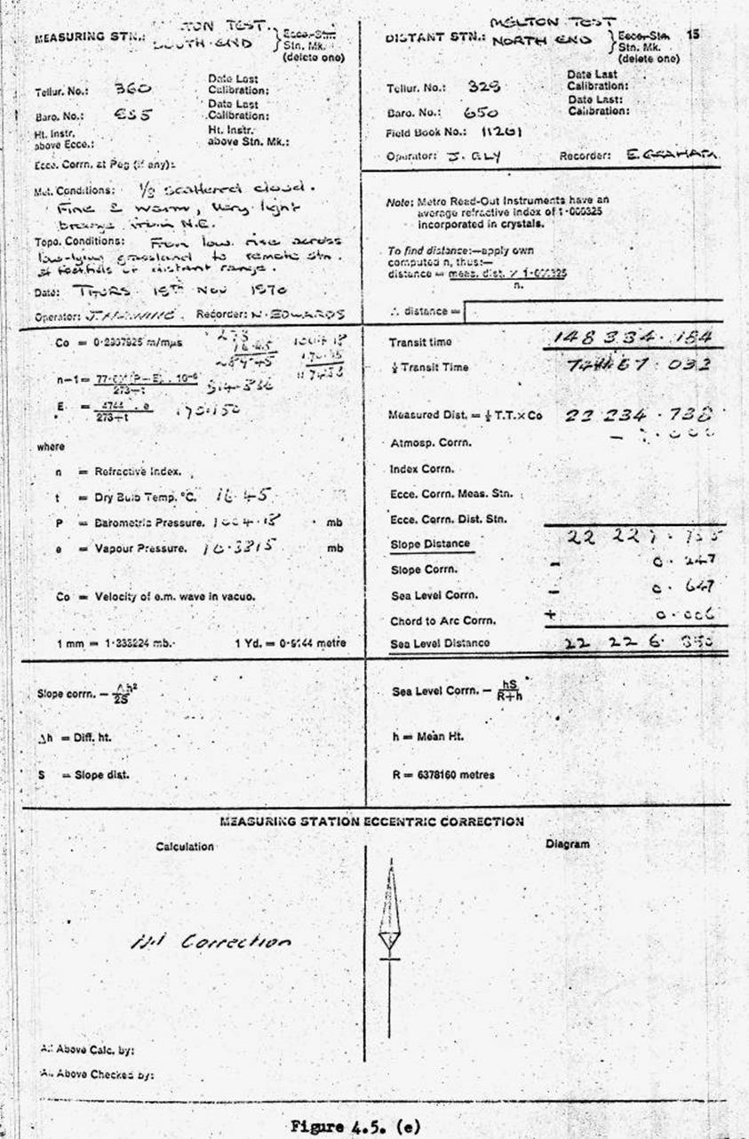
4.6. TELLUROMETER, MRA-4 – MANUAL

The manual is in PDF format.

5 The Compass

5.1.1 It is often desirable in field surveying to obtain relative directions to other points, or to find these points from given directions. Where great precision is not required, a convenient means of doing this is afforded by the “Magnetic Compass”.

This instrument has been in use in various forms and stages of refinement for many hundreds of years. In the most primitive form, the compass probably consisted of a piece of thread suspending a piece of natural magnetic ore.

At some later date, it was found that pieces of steel could be magnetised in various ways, so needles were made which could be pivoted over a divided card. Beginning with quadrants named for the prevailing winds, the card was sub-divided progressively into more and more directions, each with a specific name derived from the cardinal points, until the consequent complexity of tees system forced a change to the present method of dividing the circle into 360° numbered clockwise.

5.1.2 The Prismatic Compass

This is the normal instrument used within the Division, it consists of a thin magnetised bar, mounted on a pivot in the centre of a circular box. On the magnetised bar is mounted a circular card which is graduated in degrees with zero coinciding with the southern end of the bar.

The main features of this instrument are:-

(a) It is 1½² to 2" in diameter and is hand held.

(b) The graduations are either on a card or on a light aluminium angular ring fastened to the magnetised bar; the graduations therefore stay stationary with the bar, and the index turns with the sighting vanes.

(c) Readings are taken through a magnifying prism, attached to the outer case, and the prism reflects the magnified image of the graduations in a horizontal direction.

(d) Readings are taken with reference to the lower part of a wire in the front sighting vane, as index.

(e) The prismatic attachment consists of a 45° reflecting prism with the eye and reading faces made slightly convex so as to magnify the image of the graduations, The prism can be moved up or down, on slides attached to the outside of the case to provide adjustment for focusing the figures on the scale.

(f) Modern prismatic compasses are the liquid type. This simply means that the magnetised bar and its accompanying disk float in a special fluid contained in the case. The aim of this arrangement is to reduce wear of the pivot, and the bearing on the bar. It also helps to steady the magnetised bar.

(g) The most prolific source of error in compass work is misreading the scale, due entirely to the construction of the instrument and of the prism method of reading. As viewed in the prism, the numbered graduations increase to the left instead of the right as expected. Although the card is divided to single degrees, only every tenth is figured, so it is essential to establish between which two “tens” the bearing lies. This gives the correct “sense” in which to read the scale. For example, "62" is commonly misread as “58”. By "bracketing" the bearing, saving mentally" it lies between “60” and “70”; read “62”, no such mistake can occur.

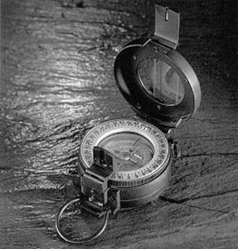
Figure 5.1.2. Prismatic Compass

5.1.3 Magnetic Declination

Earth’s magnetic field originated from electric currents in its molten core, and can be likened to a short very strong bar magnet at the centre, pointing 11° from the axis of rotation.

This means that Magnetic North, although generally close True North “declines" from it over the Earth's surface, by varying amounts which can be found, and are called the "magnetic declination" of' that place. Magnetic bearings can thus be related to True North.

Because this relationship is not absolutely constant and because of other variations in the magnetic field, and also in compass manufacture, it will be found that different compasses seldom give the same bearing for a line.

However, even in the presence of strong local attraction, all compasses will read angles between points with reasonable accuracy. In fact, "compass theodolites" using this principle, are manufactured today, so where possible this approach should be used.

5.1.4 Compass error

If magnetic bearings are required, it is sound practise to calibrate the compass to establish its "compass error" each time it is shifted to a new locality. This used to be a tedious task in un-mapped areas, but is a simple matter now that reliable maps are available for all of Australia. By comparing a compass bearing with the true bearing of an identified line as protracted from the map, or, if between trig stations, obtaining the true bearing from the station summary, a difference can be established.

If there is no real attraction, this difference should be the same as the declination of the place ascertained from notes on the margin of the map. If it is not, the disagreement is the compass error of that particular compass and should be noted. In any case the difference would include the error due to local attraction and is the amount to be applied at that particular station.

If marked on the compass case, it should be written on in pencil so that it can be altered when a change is found at a subsequent comparison, in a new area.

It is suggested that the notation be in the form "reads 2° low” rather than “-2°" which can be confusing.

As mentioned before, the compass error contains the error for the effects of the “Local Field", which will vary according to the geology of the area. Over that part of Australia where sedimentary rock predominates, it can be taken as a rough guide, that errors of more than 10 minutes will occur at 10% of locations.

5.1.5 Protracting bearings from a map

Where approximate bearings are required from a map, i.e. the 1:250,000 series, the grid lines, rather than the faint Latitude and Longitude graticules, are the most convenient from which to protract the bearings. This does introduce a small error, if the map sheet happens to be close to the Map Zone boundary. However, taking into account the general accuracy of the compass, it would only in rare cases be worthwhile to rule true meridians from the Longitude graticules, from which to protract bearings.

To obtain the magnetic bearing of a line, from the map, the true bearing is protracted, then the magnetic declination added or subtracted from that true bearing, to give the magnetic bearing.

When declination is East:- Subtract from true bearing.

When declination is West:- Add to true bearing.

Example:- True bearing 265°

Declination East - 5°

Magnetic nearing 260°

To obtain the true bearing from the magnetic bearing, the rule is reversed:-

When declination is East:- Add to magnetic bearing.

When declination is West:- Subtract from magnetic bearing.

Probably the best way of obtaining magnetic bearing from a map is to set the protractor so that it is oriented with 0° along the line to magnetic North. Proceed as follows:‑

(a) Set centre mark of the protractor over the point from which bearings are to be read. Orient to true north by keeping parallel to the grid lines.

(b) Then mark with pencil the angle of declination as shown on the map margin, i.e. declination 5° East, mark 5° to the east of North.

(d) Magnetic bearings can now be read directly from the map.

6 Mirrors and Heliographs

6.1 Mirrors

When normal opaque targets, such as beacons or cairns cannot be seen clearly in daylight, either because of atmospheric haze or excessive distance, other means mast be used to make them visible. One such alternative is a strong electric lamp, but this requires a heavy lead acid battery to supply the power. In cloud free areas, however, a good signal can be improvised from a small hand mirror, using it to reflect the sun's rays to the desired station. This is suitable only in those cases where accurate plumbing of the light is not required, and is mainly used for proving intervisibility of points. Another use for the hand held mirror is to direct a helicopter pilot to your position in country which lacks detail.

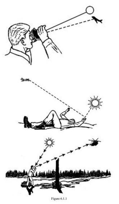
Any plane mirror of about six inches diameter, is suitable, and, for convenience, can be provided with a small central “peephole” from which the silvering has been removed. Using this mirror, it is possible to reflect the sun's rays in most directions and by adding a second mirror, to reflect a beam directly away from the sun.

By looking through the peephole, held close to the eye and aligning a small stick, or the thumbnail, at arm's length with the distant station, it is possible to shine a beam to it by centring the shadow of the peephole on the tip of the stick or thumbnail. See Figure 6.1.1.

6.1.2 The Heliograph

For observations requiring a precisely centred beam for extended periods of time, a more elaborate mirror instrument is employed. It is the military “Helio 5 inch Mk V”, a heliograph designed originally for signalling purposes. It uses one or two mirrors as required, and has an associated sighting system. See Figures 6.1.2(a) and 6.1.2(b).

It consists essentially or a circular mirror mounted on a portable tripod, in such a way that it can be rotated in both horizontal and vertical planes, about its centre, which is marked by a “dot”, a non-reflecting area about one eighth of an inch in diameter. This forms a dark. Spot in the centre of the reflected beam of light. A “radial arm” carries a foresight, or sometimes another mirror, to beam the sun’s rays in any predetermined direction.

In general, the single or “simplex” mirror set up is suitable for beaming in all directions in the semi-circle towards the sun, while the two mirror or “duplex” set up is required for the sector away from the sun. The beam from the helio is a cone with a spread of about fifty feet per mile of distance, and looks at long range, similar to a very bright star. It has been observed at more than fifty-five miles in Australia, which agrees with the rough criterion of one inch of mirror for every ten miles of distance covered.

6.1.3 Setting up the Helio

Decide whether one or two mirrors are necessary. This depends on the relative directions of the sun and of the distant station i.e. on the angle between them. If this angle is less than 120°, measured left or right from the sun, it is more convenient to use the simplex or single mirror set up, even though at 120° the effective aperture is reduced by half, and the range is thus restricted to about 25 miles. If this is acceptable the duplex or two mirror set up need only be used for the remaining 120° sector. It can, however, cover much more than this.

6.1.4 Simplex helio

(a) Assemble helio as in Figure 6.1.2(a), and plumb the tripod over the ground mark, making sure the radial arm is level by viewing it in two directions against the horizon.

(b) Direct the radial arm and jointed sighting vane towards the distant station.

(c) Rotate the mirror, by means of the horizontal adjustment screw to point midway between the sun and the distant station then tilt it with the vertical adjustment screw, so that the “dot” in the centre of the beam is brought to the centre of the cross of the foresight. This completes the approximate set up, and places the instrument in a convenient state for precise alignment.

(d) With the back of the head to the sun, look into the mirror and line up the eye with the central dot and the cross of the foresight. Locate the image of the distant station in the mirror and move the foresight until it lines on the distant station and the centre dot of the mirror. Moving the mirror will not alter the line of sight, and will achieve only a shift of the head. For very long lines the final alignment is best checked with the eye at least three feet from the mirror. Centre the shadow of the dot, which defines the centre of the reflected beam, on that part of the enamelled flap which coincides with the cross of the foresight.

(e) This completes the accurate alignment which will remain only until the dot moves off centre. As the sun moves, it will be necessary to continually readjust the mirror within every two minutes.

6.1.5 Duplex Helio

(a) Assemble helio as in Figure 6.1.2(b), and facing the sun, set the duplex mirror end of the radial arm to point 45° off the sun and on the same side of it as the distant station.

(b) Move the instrument bodilv without rotation, to a position where the duplex mirror can be plumbed over the station mark. DO NOT PLUMB THE TRIPOD CENTRE OVER THE MARK. In the duplex set up, the distant station receives the beam from the duplex mirror which is facing that station, not the simplex mirror which faces the sun.

(c) Adjust the simplex mirror, by means of the horizontal and vertical adjustment screws, so that the dot is reflected to the central mark of the Duplex mirror.

(d) Face the Duplex mirror towards the distant station then point it midway between the distant station and the simplex mirror. Now stand behind the Duplex mirror, in line with the distant station, and looking towards it, check that the simplex mirror is not in the way.

If it is, move the radial arm to provide clearance. This movement shifts the Duplex mirror off the station mark, so the whole instrument will have to be moved again, bodily and without rotation, to replumb the Duplex mirror; repeat the alignment procedure. This completes the approximate set up and places the instrument in a convenient state for precise alignment.

(e) With the back of the head to the sun, look into the simplex mirror and line up the eye with the central spots of the two mirrors. Locate the image of the distant station in the mirror and bring it into line with the two central spots by manipulating the Duplex mirror. As before, the final alignment is best checked with the eye at least three feet from the mirror.

(f) Using the horizontal and vertical adjustment screws bring the dot to the central mark of the Duplex mirror. This completes the accurate alignment, which will remain so only until the dot moves off centre. As before, the mirror must be readjusted within two minutes.

It is important to keep the mirrors clean and see that all controls are oiled and move freely. Any looseness in the head of the tripod or in the pivots or screws of the helio will cause vibration of the instrument by the wind. This in turn, prevents the distant station receiving a steady beam, or possibly any beam at all.

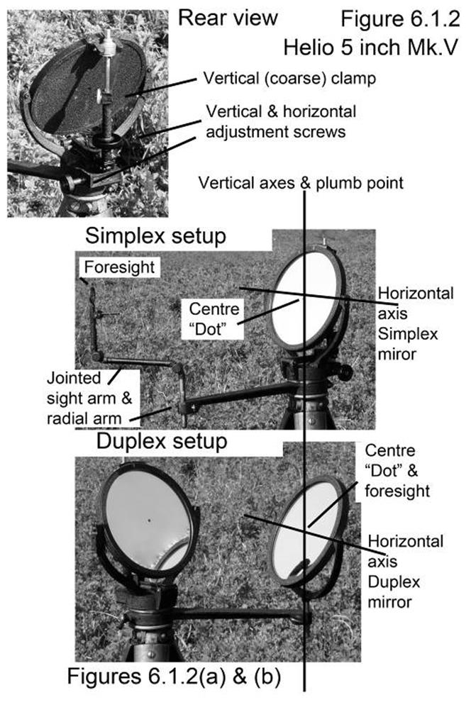
7. Station Marks and Marking

7.1.1 The station mark

This is the mark at each station, to which all coordinates, observations, and measurements are related even though the actual observations or measurements may not have been made, to or from that exact point. Over the years, these marks have been established by a number of authorities, thus there is a wide difference in the types of marks used. Mainly, the mark is a brass plaque about 77mm (3") in diameter, or a 13mm (½²) diameter copper tube, brass or stool rod, set in a concrete block. The brass plaque usually bears the name of the authority establishing the station, and often has the station name or number stamped on the surface.

Some authorities, for security often have a sub-surface mark set directly below the station mark. This is not always possible, particularly on rocky hills, however it is a wise precaution wherever possible.

Figure 7.1.1(a) shows the type of mark recently used by the Division. The GI pipe to anchor the pole type beacon protrudes about 38mm (1.5²) above the concrete block. If no beacon is to be erected, the GI pipe is dispensed with, and the 13mm (½²) copper tube used instead with its top flush with the top of the concrete block. The station number is moulded into the concrete block which is painted white, with the letters picked out in black.

Details of the above marks are supplied for information only, to help identify marks when visiting stations previously established.

Type of Station Mark previously used :

Surface mark:-

1½² diameter GI pipe (beacon anchor) with ½² diameter copper tube cemented in centre. If no beacon to be erected use only copper tube.

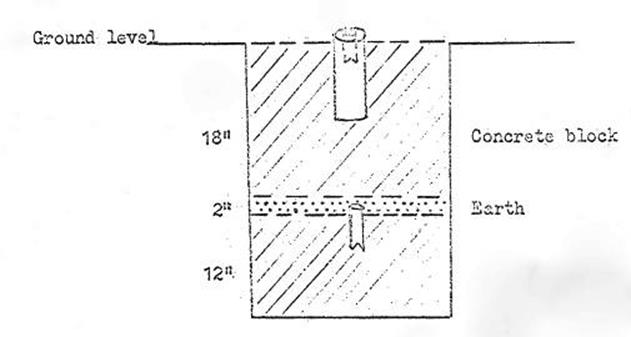
Figure 7.1.1(a)

Sub-surface mark:-

½² diameter copper tube cemented in centre of concrete block.

In most cases only the surface mark was emplaced.

The type of station mark laid down in the ''Specifications for Ground Control Surveys" will now be used at all times. Details are as follows:-

Station mark for one degree or half degree mapping control stations.

(a) The monumentation of the station shall conform, with due regard to ground surface conditions, to the specifications illustrated, guard posts shall be of in concrete to a depth of at least 0.4 metres, and painted in alternate bands of red and white enamel, 0.25m wide.

(b) Every effort shall be made to use good quality screened angulated gravel and sand. In certain areas, it may be found necessary to carry a supply of these materials.

(c) After making use of the station mark mould, the concrete structure should be neatly trowelled off, and should provide a smooth surface to conform with the shape illustrated in Figure 7.1.1(c). At this stage, while the concrete is still soft, dies of the appropriate letters and, numbers for the station should be pressed into the surface. These dies are removed as soon as the surface is firm enough. The surface should be trowelled to a hard finish.

(d) When the surface is partially dry “Boncote" ( a preparation for whitening and coating concrete surfaces) should be painted on the structure with a fexible paint brush. The impressed letters and numbers are picked cut with black paint. If time permits, a second coat of gloss paint makes all the difference to the white station mark.

(e) A circular trench four metres in diameter, 0.3m wide and 0.3m deep with vertical sides should be dug with the station mark as the centre for subsequent aerial photography. Where ground conditions prevent the digging of a well defined trench, a circle of white painted stones, four metres in diameter should be built to provide a suitable target for aerial photography. See Figure 7.1.1(e).

(f) All intermediate stations required to interconnect the one degree and one half degree stations should be marked with the standard station mark described, but only one guard post is emplanted as a witness post. No circular trench is required.

(g) If it is necessary to place a station on a sandridge, or on ground subject to erosion, the station mark should consist of lengths of 0.02 to 0.05 metres internal diameter galvanised iron water pipe, each preferably 1.5 metres long, Sufficient lengths should be coupled together and driven to refusal, so that about 0.3m of the pipe shall protrude vertically above the general surface of the ground. The number of this station should be stamped on a tag of flat galvanised iron or aluminium sheet, 0.1 metres by 0.18 metres, and not less than 1mm thick. The tag should be firmly attached by wire to the pipe. Any suitable nearby trees should be blazed and the number of the station should be chiselled on the blaze. The trees should be referenced by bearing and distance from the station mark to the blaze. Measurements should be to a galvanised roofing nail, fully driven centrally in the blaze.

(h) Where, a station of the type described in (g) is estalished, an additional satellite station will be established, which shall:-

§ Have a unique number, not a consecutive number, with that of the station on the sandridge.

· Be constructed in conformity with the standard station mark, in every way.

· Be in a safe and permanent position; in sandridge country, on the nearest firm ground; such as the flat area between sandridges usually about 200 metres from the station on the sandridge.

· Be connected to the sandridge station through a well-proportioned triangle, the third point being placed on the firm ground as a reference mark. All sides and angles of the triangle to be measured and also referred to the traverse azimuth.

7.1.2 Reference Marks

These are the marks at each station, which are placed so that the station mark can be replaced, in its exact position if it has been removed or damaged. At existing stations, various types of marks have been placed, i.e. brass plaques, copper tubes, steel rods, etc in concrete blocks.

The type of reference mark laid down in the ''Specifications for Ground Control Surveys" will now be used at all times:-

(a) Reference marks shall be three steel star pickets, (fence droppers) each of approximately 1.5m in length, driven flush with the ground, or to refusal, and cut off flush with the ground.

The picket should be surrounded with a collar of concrete 20cms in diameter, and not less than 15cms deep, with the upper surface flush with the top of the picket. The tops of the pickets should be centre-punched for exact reference measurements. Normally two of the pickets should be placed exactly on line to each of the adjacent stations, the third being located at a convenient point to provide maximum advantage for the recovery of the station.

Reference marks should, where possible, be placed in positions where they are least likely to be disturbed; for example under fences, and generally about 6 metres from the station. Any permanent structures (bore casings, concrete bridges, large concrete culverts, etc) should be accurately connected to the traverse station. Also connections of reasonable distance (up to 500 metres) should be made to corner fence posts and distinct angles in fence lines.

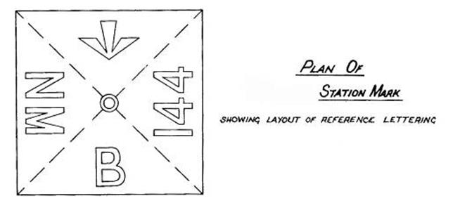
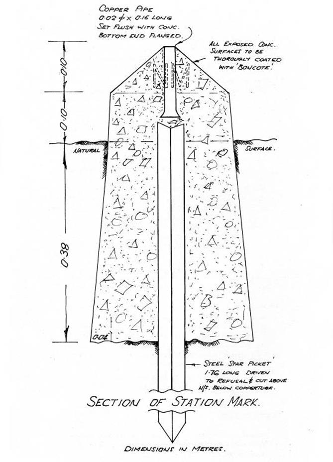
Figure 7.1.1(c). Station Mark at present in use

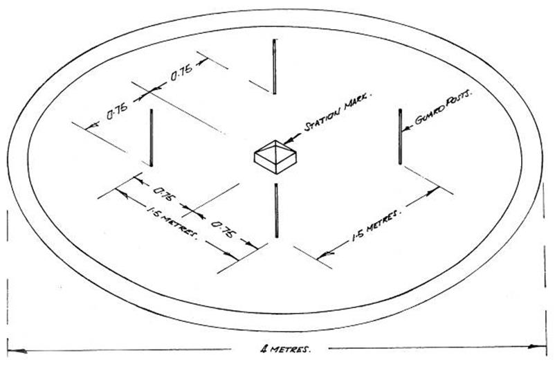
Figure 7.1.1(e)

Sketch of Station Layout – Figure 7.1.1(e)

Guard posts are 0.06m x 1.06m long and of GI pipe with “cap” on top. They are to be set in concrete, painted white with red bands 0.25m wide. The posts are placed in a square to the dimensions shown below. The sides of the square form are to be oriented north-south, east-west.

A circular trench 4m in diameter, 0.3m wide and 0.3m deep to be dug for photo identification purposes. It is important for the trench to be concentric with the station mark.

7.2 Types of Marks which have been in general use

Details of these marks are given for general interest, as they will be encountered when visiting established stations in the course of normal field duties.

Also, at some stage, it might be necessary to erect a rock cairn or beacon, or lay out a base line to establish a recovery mark very accurately. In this event, the following notes should be most useful.

7.2.1 Witness Posts

While these could be of value at all stations, they are usually placed only at stations where no large cairn, beacon or tower, which can easily be seen, has been erected. The post is either about 50mm diameter GI pipe, or 75mm square timber. It is usually painted white with the name or number of the station in black. The post would be about 1.2 metres long with about 0.6 metres out of the ground. A measurement is taken from the station mark to the base of the post, and a direction from the RO, is observed.

7.2.2 Reference trees

In timbered country, a shield is often cut in a large, solid, tree and the station number cut with a chisel in the shield. If the shield is then painted a bright red, with the station number picked out in yellow, a very good "witness post" and "reference mark" which will last for many years, has been established.

7.2.3 Recovery mark at First Order stations established on a sandridge

To be read in conjunction with 3.5.3.

The term Recovery Mark and Reference Mark are often, and probably quite correctly, taken to mean the same thing. However, within the Division, it has come to be accepted that those marks close to the station are Reference Marks, and those marks set on firm ground some distance away, are Recovery Marks. The establishment of the First Order Recovery Mark involves quite a lot of work, normally 4 men for about 2 days, and needs additional equipment to that which is usually carried.

The following method was employed to establish First Order Recovery Marks:-

(a) A point was selected on firm ground about 200 metres from or as close as possible to the station mark.

(b) A temporary mark was made, the theodolite set over it, and two base lines just over 200 yards long, at right angles to the line Recovery Mark-Station Mark were marked out.

(d) When the line had been fairly well cleared, the Recovery Mark was set in. Usually a post-hole digger was used to make a hole about 2½¢ deep. The top 1½¢ was cut square with a narrow shovel, and a 5¢ by 1½² diameter G.I. pipe was driven to within about 2² of ground level. The hole was filled with concrete to ground level, and the station number, with the letters RM, was moulded into the concrete. The pipe was filled with earth, and a ½² diameter copper tube was set in cement in the top of the G.I. pipe.

(e) Set a theodolite over this mark. An angle of exactly 90° was turned from the station mark. An exact 300' plus 1² was laid out along this line, and a 5¢ steel picket was driven in this position to within about 3" of ground level. If unable to drive right in, or if the top of post is damaged, cut off with a hacksaw 3" above ground level. Mark point on top of post with centre punch, at exactly 90° from station mark.

(f) Turn theodolite to exactly 270° from station mark. Repeat everything mentioned in (e).

(g) Carefully, by hand shovelling, clear all twigs, bumps, etc, between each base terminal, and the recovery mark. When this is done, the recovery mark and base lines are ready for measurement and angular work.

(h) The idea is, by reading all horizontal and vertical angles, and very carefully measuring the two base lines, the distance RM-Station Mark can be calculated twice, also that with all three marks, or any one of them, the station mark can be re-located, if lost because of erosion.

(i) A circular trench 12¢ in diameter, 18² deep and 18'' wide was dug around the Recovery Mark. The spoil was piled around the outside of the trench, and if the mound is not large enough a further small trench was dug outside the mound, the spoil being added to the mound.

(j) A bush tripod of three "Y" shaped trunks about 8¢ long was erected over the recovery mark. The bark was stripped from trunks, and they were well painted with primer and two coats of white paint before erection. The station number is painted on one of the trunks.

It is not likely that such elaborate marks will be established in the future, however the general technique may be used for a base line to connect a recovery mark to the traverse station.

7.2.4 Rock Cairns

Many of the Division’s stations have been marked with a pole and vanes inside a large rock cairn. Four experienced persons can assemble and erect the beacon and build an 8¢ (about 2.7m.) diameter by 6¢ (about 2m) high cairn in about half a day, as long as there is plenty of rock available right at the site. A crowbar is necessary to lever the rock free. The following routine should be adopted:

(a) Assemble the beacon; put in the station mark.

(b) Gather plenty of rock of all sizes, leave it in a circle around but well clear of the station mark.

(c) Mark an 8' (2.7m) circle around the station mark and lay the base rocks with their outer edge just touching this line. Take care to "seat" them firmly; do not lay any long, narrow rocks around the circle as they will be unstable. These should be laid with the narrow end towards the station mark. See figure 7.2.4(a).

(d) Build a second layer of rocks overlapping the vertical joins as a bricklayer does. See Figure 7.2.4(b).

(e) Stand up the beacon, staying it with the steel bars provided, plumb with a builder’s level, and tighten the bolts holding the steel stay bars. See Figure 7.2.4(b).

(f) Fill the interior with small and medium sized rocks to the approximate height of the wall.

(g) Build the wall another two layers higher, fill in the interior, as before. The wall should taper in, slightly. A stick with various marks, should be continuously used as a gauge to keep the cairn circular, and the pole central. Stand back and "eye off” the shape of the cairn to see it is symmetrical. Again plumb the beacon with the builder’s level, and straighten pole, if necessary. After this it will be impossible to alter the angle of the pole, without dismantling the cairn.

(h) Continue in a like manner until the cairn is nearly completed. The top section needs only smaller rocks, piled as shown in Figure 7.2.4(c). This should be done without spoiling the symmetry of the cairn.

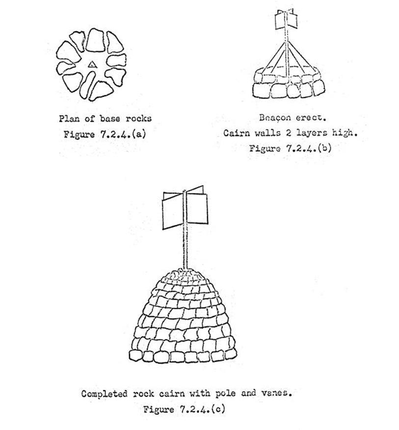
7.2.5 Beacons, Quadripod and Tripod

Some stations have a quadripod or tripod type beacon with vanes, erected over the station mark. The height to the top of the mast is about 15 to 20 feet (5-7 metres approximately).

Where these beacons exist it is possible to do the observations and measurements directly from the station mark. However, the vanes, if being observed from the distant stations, must be checked to see that they are directly above the station mark. See Figure 3.7.2 – Plumbing beacons.

The erection of these beacons is fairly straight forward; plans of the exact beacon use, would be required for assembly and the positioning of the anchor points.

All exposed station marks should, where possible, be covered with a small cairns of rocks. Reference marks should not be too obvious in case of vandalism; any authorised person will soon locate them when equipped with a station summary and measuring tape.

As stations have been established by various authorities, the type of station marking, types of reference marks, and even units of measurement, will vary considerably throughout Australia. Measurements may be in feet and inches, feet and decimals of a foot, links, or metres.

8. Erection of Towers and Mills Scaffolding Observing Platforms

Observing towers with Mills scaffolding observing platforms have been necessary in the past, and no doubt, may have to be resorted to for certain types of terrain, in the future.

The towers used have been 20 or 30 feet (6.096 or 9.144m) tripod type, windmill towers, with special adjustable "feet" to accurately plumb the tower "head", which takes the instruments, over the station mark.

8.1.1 Stand point for the Tower

The observing towers are set on, and bolted to, concrete blocks about 0.3m by 0.3m by 0.45m deep. Dimensions for positioning these blocks and bolts relative to the station mark are shown in Figure 8.1.1(a).

A level or theodolite should be used to ensure that these blocks are on the same plane, so that the tower head will be central above the station mark. If many towers are to be erected a template can easily be devised to position the blocks quickly and accurately. Blocks are usually reinforced with one or two 0.45m steel posts driven into the bottom of the hole. At least 24 hours drying is required before the tower can be bolted down.

8.1.2 Assembling the Tower

No specialised knowledge is required to assemble these towers, but it is essential to have a copy of Plan 515S, until the party becomes familiar with the task. Figure 8.1.2(a) lists the parts in a tower. It is listed in 10' (3.048m) bundles, as the towers are delivered.

Method of assembly:-

(a) With the base of the tower somewhere near the station mark lay the parts of the tower on the ground, as it will go together.

(b) Assemble one side of the tower, flat on the ground without tightening the bolts.

(c) Assemble the other two side of the tower, working from the top downwards. It may be necessary to "shake" the tower so that the bolts their respective holes. A round file is handy to clear, or enlarge, some bolt holes.

When the tower is assembled add footplates and tighten down all bolts. The bolts holding the footplates should be so positioned in their slots that the same amount of adjustment, up or down, is available.

8.1.3 Erecting the Tower

Four strong men can erect a thirty foot tower, if two of the feet are securely anchored to prevent slipping.

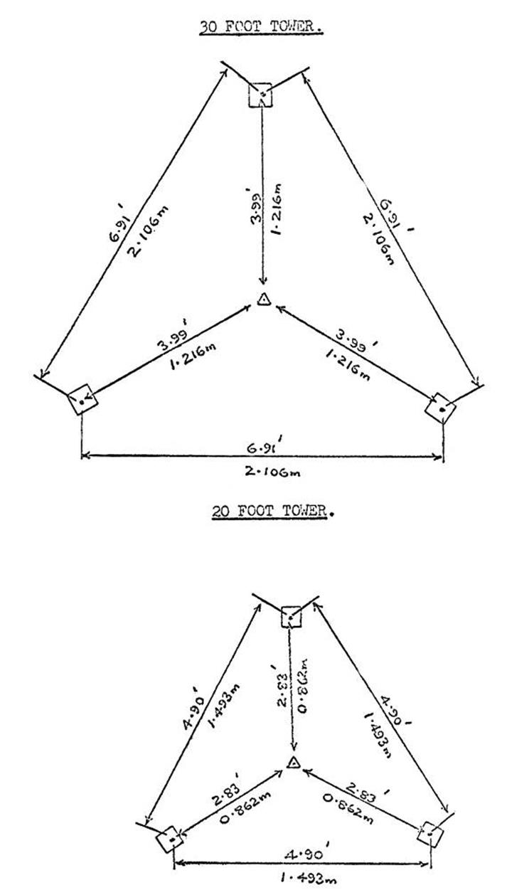
Figure 8.1.1(a)

30 FOOT (9.144m) OBSERVING TOWERS
Bundle number 1:- (top 10 feet, 3.048m, or 10 ft tower)
Main angle	Length 10 feet	3
Girts	10ft 11 7/16²	3
Girts	10ft 23 15/16"	3
Braces	5 ft 2 13/16"	6
Top ties	5 ft 4"	3
Bundle number 2:- (Second 10 ft. 1 & 2 make 20 ft tower, 6.148m.)
Main angle	Length 10 feet	3
Girts	2 ft 11 7/16"	3
Girts	3 ft 11 15/16"	3
Braces	5 ft 2 7/16"	6
Braces	6 ft 0 7/8"	6
Bundle number 3:- (Bottom 10 It 1,2 & 3 make 30 ft tower, 9.144m.)
Main angle	Length 10 feet	3
Girts	4 ft 11 7/16"	3
Girts	5 ft 11 15/16"	3
Braces	6 ft 4 9/16"	6
Braces	7 ft 4 11/16	6
Sundries:-
Tower feet		3
Bolts 1" x 3/8" UNC –HTS		12
Bolts ¾” x 3/8" BSW		21
Bolts 1" x 3/8" BSW		60
Bolts 6" x 5/8" BSW-HD		3
Washers standard 3/8"		72
Washers standard 5/8"		3
Weights:-
A twenty foot tower weighs 198lbs, and a thirty foot tower weighs 308lbs. They take up little space, only three 10feet long compact bundles per tower.

Figure 8.1.2(a)

Method:-

(a) Move the tower so that two of the feet are close to their concrete anchor bolts. Securely tie each of these feet to a bolt, passing the rope through the hole in the footplate. Lift the head of the tower and "walk" forward pushing it up.

(b) Nearing the half-way position, the weight begins to tell so one man runs to the tower base and throws his weight on to the foot which is not resting on the ground, thus helping to drag the tower upright. As the weight eases, he steadies the tower and gently lowers the foot to the ground.

(d) The tower is approximately plumbed as explained in 3.7.1. The final, accurate plumbing must wait until the erection of the scaffolding and the attachment of the tower head.

8.2 Necessary Tower Attachments

The tower head, upon which the theodolite or tellurometer is mounted is carried in a separate box. Certain other attachments which are necessary for tower observations are also required.

8.2.1 Tower head

The former traversing tower head has been modified, and simplified, so that the top plate only, is used. It fits directly on to the top of the tower with three brackets; there is sufficient adjustment at the tower feet, coupled with a small amount in the top brackets, to easily plumb the head over the station mark. The new brackets give the single top plate much greater stability, thus the theodolite is much easier to level, and will hold its level for longer periods. Figure 8.2.1(a) gives an exploded view of the tower head and brackets, and is sufficiently clear to indicate the method of attachment.

8.2.2 Protection of the Tower from sun and wind

Towers have to be protected from sun and wind during observations. Hessian screens as shown in Figure 8.2.2(a) can be easily made if time permits. If many towers are to be used, they definitely should be made. Where only a couple of, towers are to be occupied, strips of hessian straight from the roll can be used. Ropes are attached by gathering the hessian in a bunch; two strips of 6ft wide hessian are required for each side, and usually it is sufficient to shield three sides at the most. An eight foot square of hessian or canvas is required to roof the scaffolding. This is better than trying to bring the side strips over the top, to also act as a roof.

8.2.3 Useful attachments for Tower observations

(a) If lights are to be observed in the daylight, it is necessary at some angles of light, i.e. when the sun shines directly on the hessian, to have a black backing cloth behind the light, otherwise it disappears against the straw coloured hessian. These strips of black cloth should be about 8 feet wide by 3 feet deep and matte black not glossy.

(b) Figure 8.2.3(b) shows a fitting to attach a Lucas light to the scaffolding, so that the light can be shown from a position on line to the distant station.

(c) Figure 8.2.3(c) shows an adaptor to attach a Lucas light to the theodolite position on the tower head, so that a light can be shown from a position directly over the station mark when that station is not occupied.

(d) Figure 8.2.3(d) shows an adaptor to the above fittings for attachment of a "flamethrower" type light (or helio for vertical angles only).

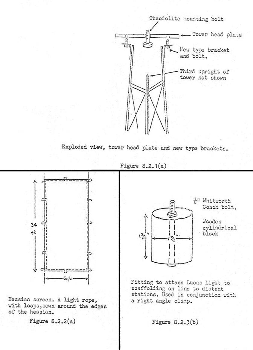
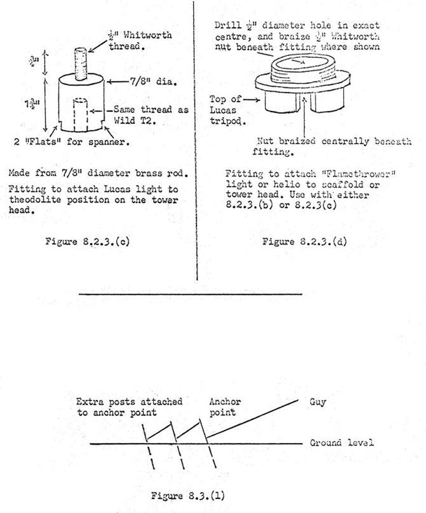
8.3. ERECTING A MILLS SCAFFOLDING OBSERVING PLATFORM (30ft TOWER).

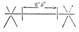
(a)	From 9 feet lengths of tube make up 24 with right angle clamps 8 feet apart. This is done by first constructing a "jig² from one 9 foot length and six very short lengths. These 22 lengths will now be called standard horizontals. (See diagram "a" for sketch of "jig").	Figure “a”
(b)	Take three 11 foot lengths (2 for uprights, 1 for a diagonal) and two standard horizontals. Form bottom side of the scaffold as shown in "b1". From same amount of material form "b2". Note that the diagonal is on the opposite slope. As these are assembled on the ground, the standard horizontals are kept as far apart as possible, while in all other stages of erection they can only be placed about 5 feet apart.
(c)	Mark a 1.724m (5.66ft) radius circle in the earth around the station mark; level site, and roughly position the foot plates so that the scaffolding will go up at right angles to the setting sun, and centrally over the station mark. Keeping the scaffolding at right angles to the sun makes for ease of shielding, later on.
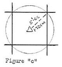
(d)	Stand “b1" and "b2" on opposite sides of the station mark, and join with standard horizontals and diagonals. Note that all standard horizontals and diagonals are on the outside. (See Figure "d”). At this stage position foot plates firmly beneath each upright, and by standing back and using a plumbob, check that the scaffolding is vertical. Adjust if necessary.
(e)	Although the scaffolding can be erected without them, two planks are of great assistance. Lay these on the top horizontals and stand four eleven foot uprights in position. Continue erection for two more horizontal levels. As previously mentioned, these are about 5 feet apart. (Chin height is a rough guide).
(f)	Five men are the ideal team, one man at each upright and the other man to pass up tubes as required. These are hung on the horizontals by resting the clamp on that horizontal.
(g)	The next horizontal level supports the platform, and its height is governed by the height of the tower and the height of the observer. However, the whole, platform can be adjusted, when complete, if within about 8 inches of its correct position. Two standard horizontals are attached to the uprights, on the inside, this time. Four horizontals(clamps slightly closer 8 feet) are laid across to support the bondwood platform. These are only lightly clamped at this stage, as they will need adjusting to suit the platform, later on. (See Figure 8.3).
(h)	The last four diagonals take full advantage of the 11 foot tubes, by placing the clamps almost at the extremities.
(i)	Two standard horizontals are clamped on the inside, at waist height above the platform, and two with clamps slightly closer are clamped across these some eight inches in from the uprights. These form the girth rails, the idea of bringing two of these rails eight inches inside the uprights is to cut down the space on the observing platform, for safety reasons.
(j)	Four standard horizontals are clamped just below the top inside of the uprights. One 11 foot length (for gantry) and one 9 foot length are clamped horizontally across the top to hold the canvas or hessian roof.
(k)	A pulley is clamped on the gantry, bondwood platform hauled up, and laid on the supports which are now adjusted to the holes in the platform. These supports are now clamped down firmly, and the bondwood platform tied to these supports.
(l)	The scaffolding must now be stayed with four guys. Right angle clamps are ideal for attaching the guys to the 4 uprights. The guys at present in use are made from good quality steel cable with stainless steel rigging screws for tensioning. Stainless steel fittings are also provided for attaching the guys to the right angle clamps and to the steel fence posts. The guys were made so that one can be attached to each twenty foot scaffold upright at platform level. To gain the extra length required for a thirty foot scaffold, two guys are joined together. Five foot steel fence posts are used as anchor points, and should be driven deeply into the ground. Where there is any doubt about the hold of these posts in the ground, an additional post or posts should be used to strengthen these anchor points. See Figure 8.3(l). It must be remembered that when the scaffold has the hessian screens attached, there is a tremendous strain on the guys in even a moderate wind.
(m)	If observations for azimuth on sigma Octantis are to be undertaken at least one of the horizontal lengths forming the roof will have to be dispensed with, and the gantry will have to be to the east or west and clear of the traverse lines.
(n)	Requirements for a thirty foot Mills scaffolding observing platform:-
	Tubes. 11 foot:- 12 for uprights. 16 for diagonals. 1 for gantry 9 foot:- (with right angle clamps 8' apart) 16 below platform 2 at platform 2 at girth 4 at top (with right angle clamps a little less than 8' apart) 4 support platform 2 at girth 1 at top	Sundries. 8 End to end couplers. 64 right angle clamps. 32 swivle clamps. 4 foot plates. 1 pulley with 70 ft of heavy rope. 8 guy wires with rigging screws and fittings. 4 steel fence posts (at least).
(o)	Weight of scaffolding : Complete scaffolding for a thirty foot observing platform weighs about 1100 lbs. It is a bulky awkward load to fit on a vehicle. Even when completely un-assembled, four thirty foot scaffoldings leave little room to spare on a Bedford 5 ton truck. Where a long tower traverse is being undertaken, it is essential to have two of these vehicles for shifting the scaffolding forward.

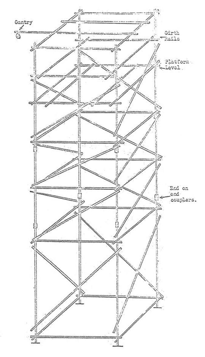
Figure 8.3. Observing Scaffolding (30 foot).

9. Access Notes and Sketches

9.1 General

In order to enable a Mapping Control Station to be readily revisited at a later date an access sketch is required to supplement the detail shown on the map.

This sketch may vary from just a "cut out" of a section of the map with the exact location of the control point plotted, to a very detailed sketch necessary for locating points in remote areas where mapping detail is scarce.

These sketches are usually compiled from speedo and compass traverses supplemented with notes. These notes should be comprehensive so as to avoid relying on the memory when drawing the sketch. Remember, some data from the notes may be omitted if considered unnecessary on the sketch, but data from the memory, which might not be completely accurate, if shown on the sketch may mislead the user.

9.2 Field notes of the speedo and compass traverse

Vehicle mileages to 1/10th mile and magnetic bearings are taken along the route at road or track junctions, bends, creek crossings, gates, fences, signposts, tanks dams, windmills, homesteads, airstrips and bridges etc.

The start point for these mileages should be at an easily located place such as a road junction, P.O., airstrip, homestead or bridge, etc.

Where access is difficult owing to poor tracks or featureless country, piles of stones and blazed trees are helpful to mark the route, particularly if time is taken to paint them white or bright yellow. Plastic streamers are useful for a brief time, but naturally cannot be relied upon for long periods.

When the vehicle cannot be driven right to the station and a walk or climb is involved, the track should be clearly marked, and any features such as streams and cliff faces encountered en route, recorded. An estimate of the time involved in walking to the station and type of walk involved, should be noted, i.e., "With 40lb load, 20 minute walk across rocky, scrub covered ground, thence 40 minutes steep climb along the ridge running NE, through Lantana, to summit. Brush hook considered necessary to cut walking track."

When camped at the base of a hill it may be necessary to descend the hill at night, after completing astronomical observations. If such is the case, the track should be marked clearly with white tape spaced at such a distance that each piece of tape can be picked out with a torch, from the preceding one. Remember it is very easy to lose a track among bushes and trees at night; tracks that appear easy to follow in daylight can become very confusing when seen by torchlight.

Figure 9.2.

There are various methods of recording field notes, probably the clearest is to draw a central column in a note book and record, between the lines, and starting from the bottom of the page, the running mileages and magnetic bearings of the route being traversed.

On the page to the left of the double lines record all detail sighted on that side of the route and on the right side notes of all detail on that side of the track. This method allows plenty of space for recording detail, and the notes are easily followed.

When taking notes for a very straightforward sketch where little detail other than road bends, gates and dams etc., is required, mileages can be written in a line across the page, each mileage having immediately after it, in brackets, notes of the detail at that point, i.e., 00 (Hillside P.O. go 296° along Pacific Hway), 4.6 (grid 242°), 5.9 (S.P. Jonesville 69m, Port Dundas 20m), leave H’way, go along Pt Dundas road, 174°) etc.

Figure 9.2 is an example of column type notes.

With good, clear field notes the sketch can be drawn so that little in the way of explanatory notes need be attached. Notes on the sketch should be confined to an explanation of problems likely to be encountered, rather than "Proceed along Pacific H’way from Hillside P.O. on a bearing of 296°, passing through a grid at 4.6, etc. The sketch should clearly show this information at a glance.

The notes, on the sketch, should show such items as rough or dangerous sections of the track, likely boggy areas after rain, climbing time on foot, and particularly a description of the feature on which the control point is located. In areas of heavy regrowth, details of the date of clearing lanes and the cutting of tracks should be noted, together with an estimate of the time that they will be useable before being overgrown.

9 3 Drawing Access Sketches

These should be drawn as soon as possible after the field notes have been taken. As seldom more than 1 station per day is selected when on reconnaissance, no difficulty should be experienced in drawing a sketch that evening, while all details of the day’s work are still clear in the mind. There is no more tiresome task than having to draw some 10 to 20 sketches in a batch, at some later date. However, the field notes should contain full details so that sketches can be drawn at any time in the future, or by another person, if necessary.

When drawing access sketches the following principles should be observed:‑

(a) All detail should be oriented with North to the top of the page, and a north point shown by an arrow.

(b) It should be stated that the bearings are magnetic, and that the sketch is not to scale.

(c) The sketch should not be cramped, but should be open and easy to read; some of the less important details recorded in the notes may necessarily be omitted to achieve this.

Conventional signs used on Access Sketches

The following signs are some of the main ones used in Access Sketches. These are normally bolder than those used on maps.

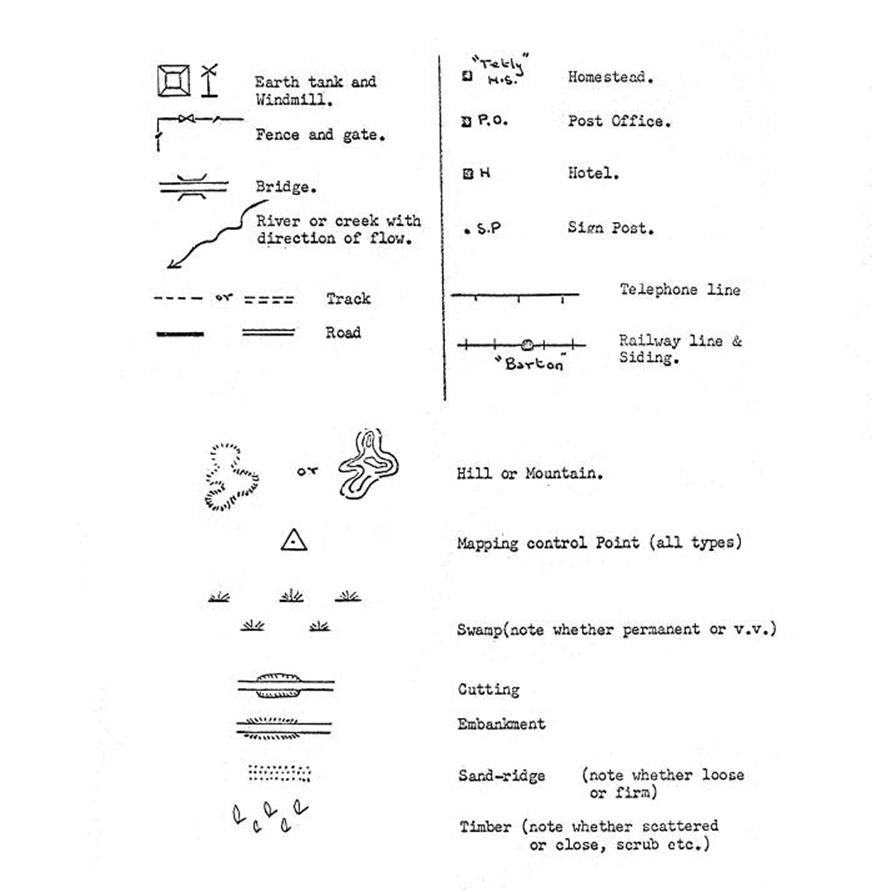
9.4 Helicopter Access

Notes on access made by helicopter should include a description of the control point, along with a bearing and distance from any prominent features. Descriptions of the helicopter pad and other useful data should all be noted, along the following lines:—

"Access was made by helicopter from Higginsfield Airstrip. The station is situated on a high, windblown sandridge, covered with light scrub. Initial access was by sky-jinnie to clear scrub and construct pad. The actual set down point was constructed from logs flown in from Higginsfield. Regrowth could be expected to make the pad unserviceable by 1971. If a sky-jinnie is not used the nearest alternative landing point for the helicopter would be about 1 mile west of the station, with a difficult walk through scrub and rain forest."

10. Map reading, including Elementary Aerial Navigation

10.1 Object of Map Reading

This is to render possible the clear and accurate visualization of the ground, so that this knowledge can be used for whatever task comes to hand. To reach this standard the student must understand the following:‑

(a) The information shown in the margin of the map.

(b) The names by which features are known, and technical terms used in mapping.

(d) Map symbols.

(e) How to visualize relief from contours.

(f) The difference between true, magnetic and grid north.

(g) Australian map grids.

(h) The use and reading of Grid (or Map) References.

It must be remembered that few, if any, maps can be perfectly accurate owing to the time lag between the original aerial photography and the first printing. Although the terrain has been mapped accurately from the photography constant alterations and additions to the man-made detail in well populated areas soon renders the best work out of date.

10.2 Understanding maps

(a) Marginal information. This varies with the scale of the map, and its purpose. It also varies slightly with the publishing authority. The information on the margins of the two scales of maps at present generally used in the field is as follows:-

(i) ICAO 1:1,000,000.

Name and number of the area.

Scale.

Elevation unit (ft), and elevation conversion scale (metres).

Projection.

Hypsometric (Elevation) Tint code.

Topographic base reliability diagram.

Scales, Nautical miles, Statute miles, Kilometres.

Edition number, compiled by, drawn by, and printed by.

Date of Aeronautical, Topographical, and Isogonic (Mag. Dec.) Information.

In addition, much information is printed on the back of the ICAO. This includes symbols for the type of aerodromes, air navigation lights & beacons, marine lights & code, also miscellaneous information such as, Isogonic lines, radio heights, prohibited or restricted, areas, etc. These are printed in dark blue on the face of the map. Hydrographic symbols (pale blue on the map), relief contours or hatchuring (brown on map) and mapping symbols (black on map), are also shown.

(ii) The 1:250,000 map series will probably be the one most used for field work in Australia for some years. The following information will be found in the margin:-

Map name, number, series & edition.

Scales in statute miles, nautical miles & kilometres.

Method of elevations shown & datum.

Projection and horizontal datum.

Details of TM grid, zone & spheroid.

Method of giving a map reference.

Magnetic declination information.

Map reliability diagram, and map sheet location diagram.

Map symbol legend.

Date of aerial photography and compilation.

Authority responsible for compilation and printer.

Two important factors to notice about the 1:250,000 map series; firstly that some map areas have been compiled by different authorities making for some slight differences in layout and style, and secondly, on these maps the Australian National Grid, in yards and using the Clarke 1858 Spheroid, is still in use. As the new 1:100,000 series is compiled, so also will be the new 1:250,000 series based on the metric Australian Map Grid and the Australian Geodetic Datum. The Universal Transverse Mercator Projection is used.

(iii) Marginal information on the 1:100,000 map series is similar to the 1:250,000 series, but enlarges on it along the following lines:-

Road classification shown.

True, Magnetic and Grid North shown in diagrammatic form.

Information about contour intervals.

Conversion table, metres to feet.(to convert metric heights to feet).

More specific information about accuracy of horizontal control.

(b) Names by which features are known and technical mapping terms.

Basin: A small area of level ground surrounded or nearly surrounded by hills. Or a district drained by a river and its tributaries.

Saddle: A neck or ridge of land connecting two mountains or hills. It is lower than the points it connects and higher than the surrounding plains and valleys.

Crest: The general line formed by joining the summits of the main ridge of a chain of mountains. Or the top of a mountain, or hill.

Dune: A hill or ridge of sand formed by the Wind.

Estuary: The tidal mouth of a river.

Escarpment: An extended line of cliffs or bluffs.

Foreshore: That portion of the shore between high and low water et maximum spring tides.

Gorge: A rugged and deep ravine.

Knoll: A low detached hill.

Main Feature: Those important features such as ridges, drainage systems, etc., which determine the shape of the terrain.

Pass: Narrow passage through mountains or hills.

Plateau: An elevated plain.

Gully: Also Re-entrant. This is where the hillside is curved inwards towards the main feature. They are always found between two spurs.

Spur: A projection from the side of a hill or mountain generally with a decreasing gradient.

Watercourse: The line defining the lowest part of a valley, whether occupied by a stream or not.

Watershed: A ridge of land separating drainage systems; the summit of land from which water divides and flows.

Undulating ground: Ground which alternatively rises and falls gently.

This list does not profess to be exhaustive. There are many common words such as hill, mountain, river plain, island cliff or ravine, etc., which it is not necessary to define.

Technical mapping terms:-

Bearing: True bearing is the clockwise angle from the true north line to the point observed.

Magnetic bearing is the clockwise angle from the magnetic north line to the point observed.

Grid bearing is the clockwise angle from the grid north line to the point observed.

Contour: This is an imaginary line on the surface of the ground at the same height above sea level throughout its length.

Contour Interval: The difference in level between two adjacent contours.

Datum Level: The level to which altitudes are referred.

Detail: All minor natural or artificial features.

Fixed Point: A point which has been joined to one or more of the main control points by traverse, intersection resection, etc.

Form Line: An approximate contour; a sketch contour.

Grid: A system of East-West and North-South parallel lines which represent progressive distances east and north of a fixed point of origin.

Grid North: The Central Meridian of a Map Zone points both true north and grid north. Within that Map Zone any line drawn parallel to the Central Meridian points grid north. The greater the distance east or west of the Central Meridian, the larger the convergence from true bearing. This is known as Grid Convergence.

Hachuring: A method of representing hill features by shading in short disconnected lines drawn directly down the slopes in the direction of the flow of water from the slopes.

Horizontal Datum: The datum to which the horizontal control is related.

Latitude: The Latitude of a place is expressed in degrees, minutes and seconds of arc, north or south of the equator as the case may be. Lines of equal Latitude are parallel to the Equator hence "Parallels of Latitude".

Longitude: The Longitude of a place is expressed in degrees, minutes and seconds, east or west from the Meridian of Greenwich, as the case may be.

Magnetic Declination: The amount Magnetic North declines from True North, at any place. It is called East or West declination according to whether magnetic north is East or West of true north from that place.

Orienting a map: When a map, sketch, air photo or plan is placed so that its true north line points true north the map is said to be "oriented".

Plotting: The process of recording on a map or plan, the field observations and measurements.

Resection: A method of fixing the position of the Observer by drawing lines to, or observing bearings to, at least two previously fixed points.

True North: This is the direction of the North Pole from the observer.

Vertical Interval: This is the vertical distance between two contours.

The word "scale" means the proportion which the length between two points on a map bears to the horizontal distance between the same two points on the ground; thus if the distance between two houses on the map is one inch and the horizontal distance on the ground is one mile, the scale of the map is one inch to one mile. This can also be expressed as a Representative Fraction. This expresses the denominator of the fraction in the same unit as the numerator; thus the R.F. for one inch to one mile is expressed 1:63,360, there being 63,360 inches per mile. As the metric system comes more into use, more scales will be expressed as a Representative Fraction.

Protracting bearings from a map has been fully described in 5.1.5.

(d) Map Symbols (Conventional Signs)

For ease of recognition, these are suggestive of the object represented. Thus the sign for a windmill could scarcely be taken for anything else as also a cross for a church and an aeroplane for an airstrip. The scale of the map governs the space available, therefore a set of map symbols is designed for each map scale. However, little trouble is experienced in understanding the variations encountered.

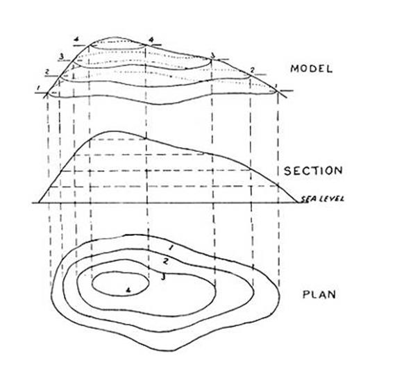
Figure 10.2(a).

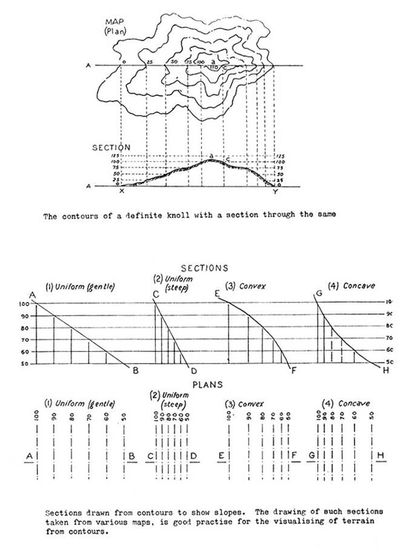
Figure 10.2(b) & (c).

(e) How to visualize relief from contours

Relief is mostly shown on the 1:250,000 maps by hill-shading owing to the lack of vertical control in most areas. However maps of more developed areas are contoured at 250ft intervals with layer tinting as an adjunct.

Form Lines are approximate contours and are used when insufficient vertical control is available for contouring. They show the elevation in the same manner but are not reliable for exact information.

With increased vertical control becoming available, the new 1:100,000 maps will be contoured in metres. Some have already been published, the contour interval being 40 metres with 20 metre auxiliary contours in selected areas.

The contour lines have their height printed at various places along the actual line and these contour lines, with the actual drainage pattern give the map reader the picture of relief. As can be imagined, un-numbered contours of a knoll without any drainage pattern could also be interpreted as a depression. It should also be noted that the closer the contour interval, the better the picture of relief.

Figure 10.2(a) below shows a contour plan of a knoll and section through the same. As previously mentioned, unless some other information such as heights against each contour, drainage pattern, spot heights, etc., is provided this plan could just as easily be that of a depression. Turn the page upside down and see.

(f) The difference between true, magnetic, and grid north

True north means the direction of the north pole from the observer and the direction of true north from the observers position is called the True Meridian. As the earth is spherical in shape, it follows that the Meridian of any point, East or West of the observer’s position will meet the true meridian of the observer’s position at the north pole.

Magnetic north is the direction of the magnetic pole from the observer’s position. The difference between the magnetic and true meridians is known as the Magnetic Declination of that position. Magnetic Declination varies from place to place throughout the world. Figure 10.2(f) shows the general pattern of magnetic declination over the Australian continent. Lines joining places of equal magnetic declination are known as Isogonic Lines. Owing to the slight annual movement of the magnetic pole the magnetic declination of a place varies slightly from year to year. See also 5.1.3 - Magnetic Declination.

Grid north. Map grids will be explained in the next section. For a definition of grid north it is sufficient to say that grids are rectangular and only one grid line coincides with a true meridian therefore it is only along this meridian (called the Central Meridian) that the grid points to true north. All other vertical grid lines are drawn parallel to this Central Meridian and do not point to true north, but in each case point to an imaginary point called “Grid North”. The angle between True & Grid north is called Grid Convergence and increases as the distance from the Central Meridian increases.

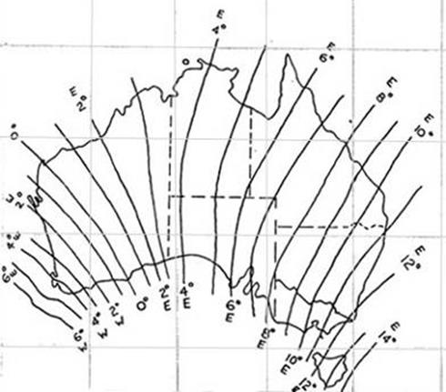
Figure 10.2(f). Isogonic Chart of Australia.

(g) Australian Map Grids

In the early 1930s the Australian National Grid on the Transverse Mercator Projection, and in yards, was adopted for Australian maps, and maps produced until the completion of the provisional and 1st Edition of the 1:250,000 maps about 1966 use this grid. Any revising to these 1:250,000 maps will be only overprints in magenta to show changes of road and track patterns, built up areas, development, etc. This grid is based on Clarke’s 1858 Figure of the Earth, and the Astonomical Coordinates of the Sydney Observatory were used as the origin. 8 zones, each 5° wide plus ½° common overlap were laid out to cover from Longitude 111°E to 154°W.

The True Origin of the coordinates of each zone in the grid is junction of Latitude 34°S and the Central Meridian of the zone. The False Origin for each zone, with zero coordinates is 400,000 yards west and 800,000 yards south of True Origin. This is to ensure that coordinates for all points within the zone will be positive.

In 1965, the Australian National Mapping Council adopted a new grid, the Australian Map Grid. It is a metric grid based on the Universal Mercator Projection and the Australian Geodetic Datum. 12 zones, 6° wide plus ½° common overlap are used to cover the Australian continent and Territories under its control.

True Origins are the junction of the Central Meridian of each zone with the Equator. False origins are 500,000 metres west and 10,000,000 metres south of the True Origin.

Figure 10.2(g) shows the layout of the map zones under both the Australian National Grid and the Australian Map Grid.

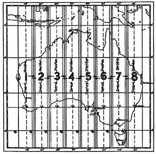
Figure 10.2(g).

Transverse Mercator Zones of the Australian National Grid.

T.O. True Origin

F.O. False Origin (400,000yds West, 800,000yds South of T.O.

Zones overlap ½° on each side.

(h) The use and reading of Grid (or Map) References

(i) The 1:250,000 Australian National Grid (yards). It will be some years before this series will be republished on the Australian Map Grid (metric), and as these maps are the basic map for current field work any grid references used will still be in yards. However, this is no problem as all maps incorporate a panel in the margin giving an explanation and an example. The black numbered grid lines indicate 10,000 yard intervals, and the Grid Reference of a point is given to the nearest tenth of this interval, i.e. 1,000 yards. Each grid line is numbered with two figures, the 100,000 and the 10,000. Thus the three figures for the Easting reference come from the two printed figures on the nearest line west of the station with the third figure representing the number of tenths the point is estimated to be east of that line.

It follows that the three figures for the Northing reference come from the two printed figures on the first grid line immediately south of the point, with the third figure representing the number of tenths the point is estimated to be north of this line.

(ii) The 1:100,000 Australian Man Grid (metric). As these maps will gradually become available an explanation of the giving of Grid References on these maps, is warranted. The black numbered grid lines indicate 1,000 metre intervals. By estimating the tenths of these intervals in the same manner as in (i) above, a Grid Reference to the nearest 100 metres is obtained.

From the margin and the Grid information panel ascertain within which 100,000 metre square the point lies, and prefix the six figure reference with the two letters nominating that 100,000 metre square. See Figure 10.2(h) for examples of Grid References on both the 1:250,000 map and the 1:100,000 map metric grids.

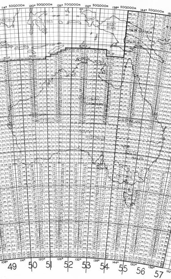
Figure 10.2(g). Zone Boundaries, noting Zones overlap ½° on each side, and selected Central Meridians, noting that the intersection of each Central Meridian and the Equator is the True Origin. False Origins are not shown.

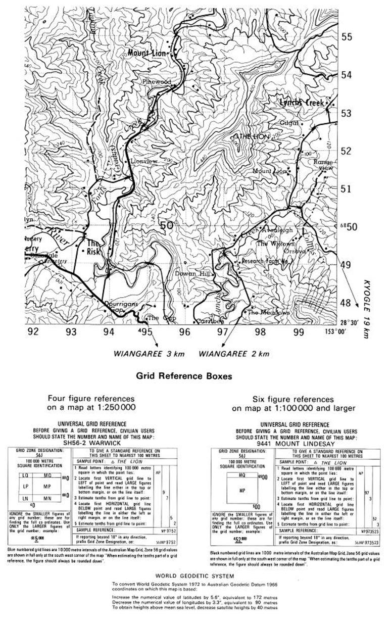
Figure 10.2(h)

10.3 Hints on Map Reading

Once a good knowledge of the amount and variety of information obtainable from the map has been assimilated, map reading itself is mainly a matter of having plenty of practise at following maps under field conditions. The following hints have been found useful:-

(a) Always check the date of the air photography, map compilation and latest amendments. These will give an idea of the reliance to be placed on that particular map.

(b) Always have a prismatic compass, protractor, and scale handy. If no scale is available make one along the edge of a piece of blank paper.

(d) Always use a soft lead pencil (not a ballpoint) to draw in bearing or make notes of directions and mileages. It is a great help to be able to quickly plot one's position, particularly when on reconnaissance. When this is done in pencil the map can be cleaned up later and the required data only plotted permanently in ink. Also always have a notebook handy for more elaborate notes.

(e) When “feeling the way” in poorly mapped country or along tracks not shown on the map, always keep, a speedo and magnetic bearing log. At the end of the day correct bearings to true and plot the days travel as accurately as possible on the map. The information gained is often necessary to help prove lines plan the next day’s moves, or to update the published map.

(f) Finding approximate north from analogue watch and sun (Southern Hemisphere) : Lay the watch flat, point 12 to the sun, north lies mid-way between 12 and the hour hand. The method is quite rough, but is often useful.

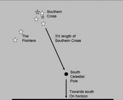
Figure.10.3(g). (Not to Scale).

South Celestial Pole is elevated above the horizon by an amount

equal to the Latitude of the observer’s position.

(g) Finding approximate south from the Southern Cross : Imagine the Southern Cross as a kite, estimate the length of the greater axis and extend this axis from the tail of the kite about 3½ times. The point reached is the South Celestial Pole, i.e. a point true south of the observer, elevated above the horizon by an amount equal to the Latitude of the observer’s position. See Figure 10.3(g).

10.4. Elementary Aerial Navigation

(a) Standard required in the field

The main requirement is to navigate a light plane on reconnaissance or Aerodist flights, or a helicopter to establish or visit Mapping Control Points.

Therefore ability to follow terrain mainly from the 1:250,000 map and air photo's is needed rather than any knowledge of radio beacons, application of drift to courses, flight plans, etc., which can safely be left to the pilot.

(b) At times it may be necessary to use the ICAO maps, but where possible the 1:250,000 series should be used. A protractor and scale (or set of dividers), are necessary. The pilot will estimate drift wind speed, etc. He will apply the drift so as to keep the correct course, altering it when necessary during flight, and will estimate his speed over the ground, in knots, from this point on, ground speed should be converted to flying time in minutes and this should be the basis of all Aerial Navigation.

Usually the pilot will be a good navigator, however the passenger will need to follow his own maps so as to perform his various technical tasks.

(c) Prior to the commencement of the flight, plot the course to be followed on the map and mark off the points as they will be reached, in time intervals.

Once the flight commences, mark the time each point is reached with a soft pencil thus enabling a close estimate of the time of' arrival at the next point of detail.

Concentration is the main keynote; if in doubt of the aircraft's position never worry about detail already passed, watch the terrain ahead and concentrate on locating some point which will positively identify your position. If on a low level flight and in doubt, immediately take the aircraft higher; it is amazing how much easier locating the position becomes at 3,000 feet above ground level.

(d) If the final approach to a point is to be made on air photos, mark the boundary of the area covered by the photos onto the map and once the aircraft reaches that boundary, follow the photographs exclusively.

(e) The 1:250,000 maps give a fair amount of natural detail even in many unpromising areas. Probably the drainage pattern gives the best navigation aid. Even in endless sandridge country a clear pattern is there to be followed by a keen-eyed navigator who can really concentrate.

(f) Most difficulty will be experienced in flat, featureless areas with no drainage pattern, or man-made detail such an earth tanks, etc.

Often a long flight across such terrain is necessary to site, or visit, a mapping control point. In this case initial preparation should ensure wide aerial coverage of the area. The aircraft’s course should be plotted to the most easily identified point on these photos, with a short separate course to the mapping control point. Once the identifiable point is located there is no doubt as to one’s position thus giving a better chance of locating the control point at the first attempt.

10.5 The Use of the Plane Table

With the plane table the detail of an area can be mapped graphically as it appears before the observer. It was used extensively prior to the adoption of photogrammetric methods. Plane table mapping over small areas has some important advantages:-

(i) All direction measurements are instantly recorded on the map. The intervening processes of recording field notes and plotting them are eliminated.

(ii) The map is constructed at once, in the field, so that no permanent records are necessary, other than the map itself.

(iii) The topographer sees the undulations of the ground that he is mapping. He can draw a good representation of the contours and he uses fewer field observations.

(a) The principle of mapping with the plane table

The plane table is a drawing board mounted upon a tripod and capable of rotation in a horizontal plane. The essence of the art of plane tabling is that the board should be so oriented that directions upon it are identical with corresponding directions in nature. When this orientation has been achieved, rays from a known point, representing directions in nature, can be drawn upon the board. By means of intersecting rays, drawn from different known positions, or by distances measured along a known direction, points of detail in the countryside may be transferred to the paper.

(b) The plane table and ancillary equipment

(i) The plane table is usually rectangular and about 18" x 24". It is made of light, well seasoned timber and has a screw thread which enables it to be mounted on a tripod and rotated or clamped in position, as required. It is contained in a canvas cover which has straps on the back for carrying on the shoulders.

(ii) The plane table tripod may be of the "Johnson Head" type which allows quick levelling of the plane table, or it may be of a very light construction with a rigid head and the plane table is levelled by the placing of the legs. The "Johnson Head" type is easy to use but is heavy to carry, the lighter type is thus probably the best for general use as one soon gets used to positioning the legs to quickly level the plane table.

(iii) The sight rule or alidade consists of a straight edge, made of non-magnetic metal, to each end of which is attached a vertical arm. One vertical arm has an eye-slot, and the other acts as a frame for a taut sighting wire. The distant object is observed through the sighting-slot and aligned against the sighting wire; thus directions in nature may be transferred to the board as pencil lines. The straightness of the ruling edge should occasionally be verified by ruling a line and then reversing the ruling edge end for end.

A parallel arm is a convenience, the edge of the rule then being positioned close to, but not on, the plotted position of the point being sighted. Once the point has been sighted, the parallel arm is moved exactly against the plotted point, and the direction drawn.

If the alidade has no parallel arm, its edge should be positioned against the plotted point by laying a pencil, on its side, with the blunt end exactly coinciding with the plotted point. The edge of the rule is kept against the end of the pencil while bringing the sight onto the distant point. Check that the rule is still on the plotted point and draw the direction.

In short the alidade takes the place of the theodolite to obtain horizontal directions.

A telescopic alidade is available, however these are cumbersome and would not normally be carried around for close detail work. Their main use would now be for contouring where the stadia marks and a staff could speed up the locating of a close network of spot heights.

(iv) The "Indian" pattern Clinometer consists of a level bubble in a frame with a vertical arm at each end, one arm contains a peephole and the other has a sliding vertical sighting wire and scale of natural tangents, to 2 places of decimals, with their corresponding vertical angles. The bubble is levelled with a thumb screw, the distant object is sighted through the peephole, and the sighting wire brought into coincidence with the object. Check that the bubble is still central and read the natural tan of the angle, estimated to 3 decimal places, from the scale. This tan, multiplied by the scaled distance from the plane table, gives the difference in height, to plane table level; correct it to ground level. From this it can be seen that the actual angle is rarely needed and therefore rarely recorded.

An Abney level can be used instead of the "Indian" clinometer with probably slightly more accurate results; however, in this case, a Table of Natural tan's of angles would have to be carried.

Before commencing field operations, the "Indian" clinometer, or Abney level, should be checked against a theodolite read vertical angle and adjusted if necessary. Further checks, during extended field operations are advisable.

(v) A good quality scale is a necessity. One graduated in millimetres and about 300mm long will now suit all tasks unless some specialized scale is required. In plane tabling, the scale lakes the place of computations for obtaining distances.

(vi) The Trough Compass consists of a magnetised needle about 6" long, suspended in a rectangular container. This is usually housed in a wooden box with a sliding lid. The closing of this lid lifts the compass needle clear of its pivot. When the orientation of the board has been established with reference to distant fixed positions, the compass is positioned on the board with its needle on the central mark; a pencil line is now drawn around the box. This pencil mark and the compass will approximately orient the board on future occasions in that area, subject of course to local attraction from fences, vehicles, ore bodies etc.

(vii) Binoculars. An average pair of binoculars of 8x magnification are satisfactory; these will be in almost continuous use.

(viii) Pencils. 2H to 6H for drawing rays, HB for making notes and calculations. Remember that in hot climates pencils soften slightly; under such conditions the 6H will appear more like a 2H. Pencils should be kept sharp; a sharpener and fine emery or glass paper are essential. A strip of the emery paper can be attached beneath the board.

(ix) Erasers (Rubbers). Both soft and hard are required. On plastic sheets the hard is more often used than the soft; no amount of rubbing seems to harm the surface of these sheets.

(x) Needles. These are required to prick through points as they are established so that they are not lost when rubbing out superfluous data.

In addition, at the conclusion of the day's work, the detail which has been finalized is "inked in". Requirements for this are a selection of colours in good quality drawing ink which is suitable for plastic sheets, a "Rapidograph" type pen with a selection of points and a good quality straightedge. A contouring pen is a great help for this part of the drawing.

Normally arrangements will have been made to have at least 3 control points established in the area. The coordinates of these points will now be in metres on the Australian Map Grid. These preparations are:-

(i) Decide on scale to be used.

(ii) Draw a rectangular grid to suit the scale.

(iii) Plot the control points on this grid.

Stable based plastic drawing material is ideal for use with the plane table. When plotted ready for field use it can be attached to the board with masking tape along each edge. This prevents dust and grit getting between the board and the sheet. If good quality drawing paper is used it should be pasted to a sheet of aluminium before plotting.

(i) The scale to be used. This is entirely governed by the task in hand. For mapping tasks 1:100,000, 1:50,000, 1:25,000, 1:12,500 and 1:10,000 are most often used. If engineering plans of camps or establishments etc are required these may be to scales of 1:1,000 or 1:500.

(ii) Drawing the grid. The first step in drawing a grid of squares is to construct a rectangle near the outside edges of the board. It is clear that once such a rectangle has been drawn, equal distances may be measured off along its sides and joined with a straight edge to form the grid.

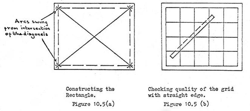
To construct such a rectangle, draw two diagonals roughly from corner to corner of the plastic sheet which has been out to the size of the board. In fact it should be cut about 2mm smaller than the board for ease of sticking down with masking tape so as to provide a perfectly flat surface.

Set a beam compass to strike off arcs of equal distances from the intersection of these diagonals. These arcs should cut the diagonals about 2 to 3 centimetres from each corner. Join these and points which will then form a perfect rectangle. See Figure 10.5 (a).

When the grid has been drawn, check its accuracy by laying a straight edge across the diagonals of the squares where it must cut all intersections. See Figure 10.5 (b).

(iii) Plotting the control. Each grid line is given its coordinate value in the same manner as a map. Then the control points are accurately plotted. A good check of the accuracy of this plotting can be made by comparing the scaled distances between these points and the actual measured, or computed, distances supplied with the coordinates.

The accuracy of the completed map depends on the precision of the plotting of the control points on which it is based. The utmost care must be taken to ensure that no error, which can be controlled, is permitted to appear.

(d) Mapping with the Plane Table

The four main methods of obtaining detail with the plane table are :-

1. Intersection

2. Resection

3. Triangulation

4. Ray and Distance

Traversing with the plane table is sometimes used. The above methods will now be described in detail, however, it is important to stress here that in all the above cases, clinometers heights should be taken and should be worked out while the board is set up. Naturally these calculations cannot be commenced until the first 3 way intersection, resection or triangulation has been completed, so that distances can be scaled. A comparison of the heights so obtained gives a check on the accuracy of the position of the new point; in the event of a large difference in the heights a check of the scaled distances, the plotting and the clinometer readings, should be made.

(i) Brief description of general procedure. All the established control points are visited and rays are taken to all prominent points of detail. The board must be set up and levelled close to the station mark. How close depends on the scale to be used and the accuracy one can plot. Under field conditions the plotting accuracy is about 0.25 of a millimetre, thus the following table gives some idea of the accuracy which can be expected.

At 1:12,500 1mm = 12.5m and 0.25mm = 3.1 metres

1:25,000 1mm = 25m and 0.25mm = 6.25 metres

1:50,000 1mm = 50m and 0.25mm = 12.5 metres

1:100,000 1mm = 100m and 0.25mm = 25 metres

If making plans at scales of 1:500: 1:1,000, etc it is necessary to plumb the exact point on the board over the station mark.

Once the drawing of rays is commenced, notes with thumbnail sketches are entered against each ray, or alternatively, the rays are numbered and the details are entered in a note book against these numbers. As mentioned previously clinometer angles are recorded.

When setting up at the first control point visited the plane table is, oriented by the identification and sighting with the alidade of one of the other plotted control point. A check of the orientation of the board and also of the office plotting is made by sighting in turn each of the other plotted control points which is visible.

To avoid a mass of insoluable rays on the board, each time a three way cut has been obtained, the point should be "pricked through" and the relevant rays rubbed out.

Once the intersecting of points from the control stations has been exhausted move through the area gathering further detail by:-

Further intersections from the new points established.

Resections from various places in the area.

Triangulation.

Ray and Distance.

"Inking In" should be a gradual process; at the conclusion of each day's work sufficient "inking in" should be done to ensure no detail is lost.

Once sufficient spot heights have been obtained contouring should be done in the field with the terrain in view. Methods are elaborated upon towards the conclusion of these notes.

The methods of obtaining detail:

1. Intersection. This is the most accurate method and thus yields the best further control points. It is easy but a few precautions should be taken:-

(a) Orient the board carefully by sighting the most distant control point.

(b) Make sure the board is properly clamped.

(d) Draw the rays in the direction of the point being intersected. Do not draw it right into the observer's plotted position or a mass of converging lines will result. Number the rays and make thumbnail sketches and notes.

(e) Check that the board has not been moved by resighting one control point.

(f) Lay trough compass on the board with needle on the north mark and draw a "box" around the compass. This "box” will be used, later on, to approximately orient the board at resection points. A check of this "box" can be made at the other control points to ensure that it was not drawn at a station where a large amount of local attraction upset the compass needle.

(g) Take clinometer heights; calculate, if distances can be scaled.

Intersections, also resections and triangulation, do not give very accurate results if the angles are small, try and keep the angles over 30° and under 150°. See Figures 10.5(c) and 10.5(d).

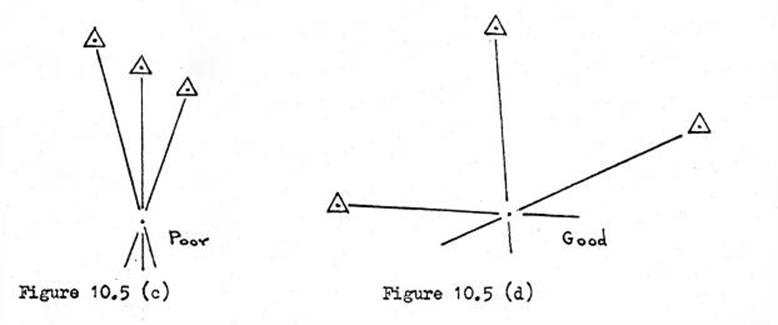
While taking as many rays as possible, the beginner should take care to avoid covering his board with a dense and insoluble network of rays.

At least 3 rays are necessary to fix positions which are to be used for subsequent control. Positions fixed by 2 rays can only be accepted for mapping detail and then only when, there is no reasonable doubt of identification. However, if a point on which a 2 way cut has been made, is visited and checked by triangulation, its accuracy is probably as good as a three ray intersection, if the angles are all over 30° or under 150°.

If the observer sees a point which he intends to visit, a ray can be taken to it. This is known as an “Azimuth Ray”. On visiting the point, the alidade can be laid along the azimuth ray and the board oriented accurately by sighting the control point. This helps considerably when doing resections. If the ray is short, a further length should be drawn in the margin as the alidade cannot accurately be laid along a very short line which, in turn, causes the board to be inaccurately oriented.

Remember that intersections possess the great advantage that they enable the points to be fixed without visiting them thus saving a great deal of time and often a great deal of walking.

2. Resection. This is the term used for the process of fixing a position from at least 3 previously fixed points, without actually visiting them.

(a) Trough Compass Method: Orient the table with the trough compass, clamp it, sight the 3 fixed points and draw back rays from their plotted positions on the board towards the observer's position which is unknown, at this time.

These rays (unless the original orientation has, very luckily, been correct) will produce a triangle on the board, i.e. the "triangle of error". This is because the orientation of the board is not accurate, and it follows that the orientation error (in angle) of each ray is the same. There are certain set rules for solving the triangle of error. Firstly there are 2 cases:-

Case 1:

If the observer is within the triangle formed by the 3 fixed points in nature, then his position on the board will be within the triangle formed by the rays on the board. His exact position within the triangle is determined by the condition that its distance from each of the rays is proportional to the length of these rays, i.e. nearest to the shortest ray, furthest from the longest ray and intermediate from the intermediate length ray. See Figure 10.5(e).

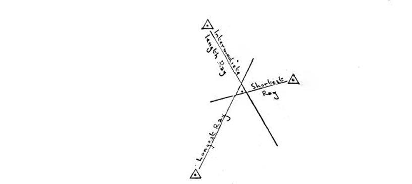
Figure 10.5(e) : The observer's position is within the triangle of error.

Case 2:

If the observer is outside the triangle formed by the 3 fixed points in nature, then his position on the board will be outside the triangle formed by the rays on the board. There are 6 sectors formed by the rays; however, all but 2 of these sectors can immediately be discarded because, when facing the fixed points, the observer’s position must be in one of the 2 sectors where all the rays are either to his right, or to his left.

A foolproof method of deciding on these two sectors is to consider the rays as 3 spears pointing away from the control stations. The two sectors in which the thumb and fingers would go to pick them up as a bundle are the sectors in which all the rays are either to the right or to the left of the observer. See Figure 10.5(f).

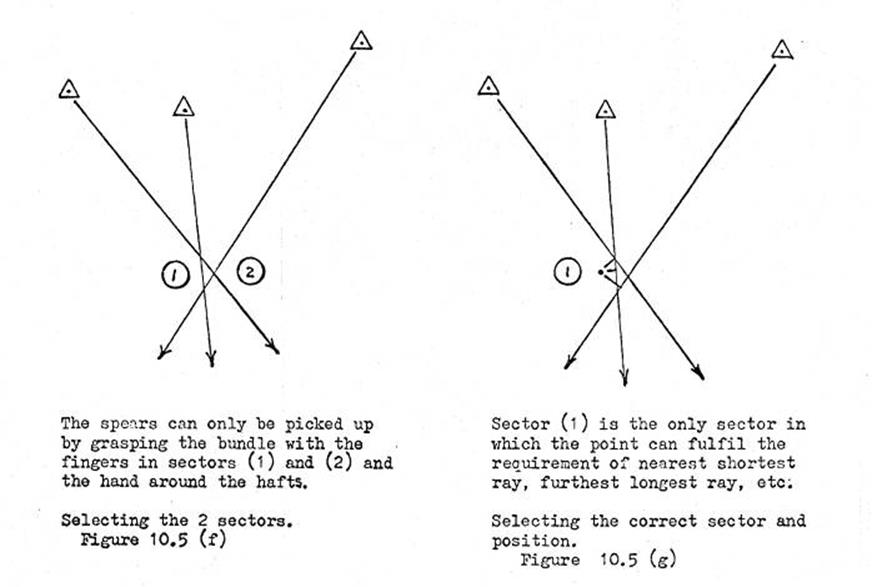
The one sector, of these two, in which the point actually lies, will be the one where it can be nearest the shortest ray, furthest from the longest ray, and intermediate from the intermediate length ray. See Figure 10.5(g).

The next step in both Case 1 and Case 2 is to estimate the observer's position on the board in relation to the triangle of error, mark it, rub out the rays forming the triangle, lay the alidade along a line from the estimated position to the most distant control point, reorient the board by sighting the control point and clamp it.

Again draw the 3 rays which now may give a perfect cut, or more likely, a much smaller triangle than the original one. Repeat the operation until no triangle is formed. Prick through and clean off the redundant rays.

Resection is most accurate when the observer's position is inside the triangle formed by the 3 control points (Case 1). If the observer's position is outside the triangle formed by the 3 control points, the best results are obtained when the angle between the extreme rays is large; 60° is rarely more than fair whilst nearly 180° is good. Obviously 180° would mean that the point is exactly on line between the 2 control points and this should give an accurate resection if the third ray cuts this line at an angle between about 50° and 130°.

Generally speaking, with control points of equal value, fix the new position from the nearest points but orient the board from the more distant points.

Once sufficient detail has been plotted, it is often unnecessary to resort to the trough compass to orient the board. A good first approximation can be obtained from plotted detail such as fences, power or pipe lines roads, etc.

(b) Tracing Paper method: A piece of tracing paper is laid anywhere on the board, which does not need to be oriented with the trough compass. Sight 3 control points in turn, drawing rays from each on the tracing paper, which must not be moved in the process. A tiny hole, about the same size as the point of the plotting pencil, is made at the intersection of the rays on the trace.

The trace is then fitted over the plane table plot in such a way that each ray passes through the plotted position of the control point to which it refers. The observer's position on the board will be at the intersection of the 3 rays on the trace; mark this position on the plane table through the tiny hole in the trace. Orient the board by sighting one control point and check with the other two control points.

The difficulty of carrying sufficient large size tracing paper and handling it in the wind detracts from the usefulness and accuracy of this method. However, particularly for the beginner it may, with advantage, be used for a first approximation which will often be the correct solution.

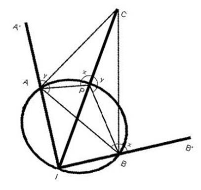
Figure 10.5(h)

(c) The Collins Point Method (Bessel’s Solution). This method is attractive in that it requires no successive approximation, and once mastered is quite quick. Consider the diagram 10.5(h), A, B and C are the control points and P is the observer's position which is at present unknown. The theoretical basis of the method is; AB is chosen as the base and the circle ABP drawn. CP is produced to meet this circle at the Collins Point I. Thus if the position of I can be located the direction of IC and therefore PC is known and the table can be oriented. In practise, the circle is not drawn.

In figure 10.5(h)

APC = x BPC = y
BAI = BPI = 180°-y

Therefore A¢AB = y

Similarly B¢BA = x

In practise it is the positions of these points plotted on the board which are used and in the following explanation lower case letters, a,b c, etc, will be used to indicate the plot and upper case letters A,B C etc, to indicate the points can the ground.

From the example shown in Figure 10.5(h); on the board the position of I is found with respect to a, b and c. Its position will be given by the intersection of the lines aa' and bb'. These lines are obtained by plotting y at a, and x at b. This is simply achieved as follows:- (Remember that the board is at P)

1. With the alidade pointing along ab turn the board until B is sighted and clamp it; this makes abB a straight line.

2. Draw in a ray from the control point not used as the base, that is from C, through the position a. This is the line a'a. The plotted point c is not used until step 6.

3. With the alidade along ba sight on A and clamp the board, this makes baA a straight line.

4. Draw in a ray from C, through the position of b. This is the line b'b.

5. a'a and b'b are produced to meet at i.

6. The alidade is laid along ic and the board rotated to sight C and clamped. The board is now oriented.

7. Rays are now drawn from A through a, and from B through b. These should intersect ic at the position p.

From the foregoing it can be seen that the board has to be clamped 3 times after sighting stations; this has to be done with care or a poor fixation will result.

A little experience is required to choose the correct base, not only to give the best fix, but also to ensure that the point i falls on the board. An interesting case arises when CP is a tangent to the circle ABP, in which case i and p coincide, though a solution is still possible.

(d) Danger Circle. All methods of resection fail when the circle which passes through the three control points also passes through or very close to, the position to be fixed. When this occurs points are said to be on the "Danger Circle" and all plane table operators should be on their guard against this possibility. See Figure 10.5(i).

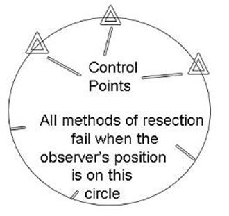
Figure 10.5(i).

3. Triangulation. When sorting out the rays from the various control points it will often be found that there are quite a few points to which only 2 way cuts were obtained.

To ensure that the same point was indeed sighted from both stations it is necessary to visit such points. Set up the board and orient by sighting one of the two control points visible along its appropriate ray; clamp and sight the second control point. If the alidade coincides with the ray originally drawn from this control point, the intersection of the rays is the accurate position of the observer, Subject of course to the triangle being well proportioned.

4. Ray and Distance. Detail close to any point established is gathered by ray and distance. At most mapping scales and over distances of 100 - 200 metres pacing is usually sufficiently accurate. It is considered that, with practise, an accuracy of ±3 metres per 100 at the very worst should be expected. No attempt should be made to pace an exact metre; pace naturally and calibrate these paces against a 100 metre chained distance. This calibration should be done in similar terrain to that being mapped.

If a person paces 114 to the 100 metres this gives 1.14 paces per metre therefore:-

Number of paces /1.14 = Distance in metres.

Minor Methods of Obtaining Detail

The "Position Line" and "Cutting; In"

This can be roughly described as a combination of intersection and resection and can be very useful in obtaining extra detail once a reasonable amount of control has been accumulated. All that is needed is to get exactly on line between 2 control points, or on the prolongation of such a line, or along the straight line of a road, a power or pipeline which has been accurately plotted.

Orient the board along such a line, sight with the alidade a control point as near to right angles as possible to this line, then the point where this ray cuts the position line is the observer's position. Where possible, sight a second control point as a check. This method is very suitable for fairly quickly obtaining extra spot heights, for contouring.

Traversing with the Plane Table

Sometimes sufficient detail cannot be obtained by the previously mentioned methods owing to timber cover or flat terrain etc.

In such cases it may be necessary to resort to traversing. It is slow and very liable to the accumulation of error, because every error of measuring distance, or of orienting the board is carried forward.

To be satisfactory the traverse must close on another control point, or be in a loop closing on the starting point. In this way gross error can be eliminated and accumulated error adjusted out. Proceed as follows:-

1. Set up and orient the board at some known point.

2. Draw a ray to a point in the required direction, pace (or chain) the distance.

3. Go to the new point, orient the board on the back ray to the point just vacated.

4. Draw a ray to another point in the required direction and again obtain a distance - and so on, until the traverse is completed.

It is clear that laying marks such as ranging poles will often be required at the rear and forward stations, making the task slow and cumbersome and a task for more than 1 person. Thus traversing is a poor substitute for any of the other methods of obtaining detail with the plane table.

Orientation of the board is entirely governed by the back ray. Such rays, when drawn must be extended by short lines near the extreme edges of the board to give maximum length for each orientation.

As the traverse will have to be adjusted it is advisable to plot it at twice the scale on a sheet of paper which has been gridded to twice the scale. This plotted traverse is then adjusted geometrically to the required length and swung into correct orientation and the resultant adjusted traverse is plotted onto the plane table. See Figure 10.5(j).

To adjust the traverse, a line A,b,c,d,e, is plotted equal to the total length of the traverse. At e, a line eE is drawn at right angles to Ae, and equal to the traverse misclosure. Draw a line joining points A and E. Perpendiculars are then drawn to meet this line from the intermediate points b,c and d. The distances bB, cC, dD and eE are the adjustments to be made to the field plot of the traverse. The direction of these adjustments is parallel to that of the original misclosure at E.

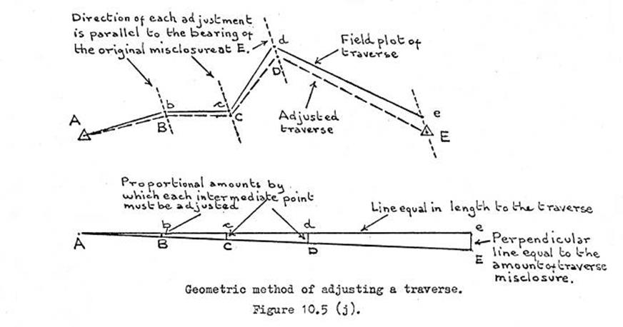
Figure 10.5(j). Geometric method of adjusting a traverse.

Contouring with the Plane Table

A network of spot heights must be built up to cover the area and no control point should be established without obtaining a height. The density of the coverage depends on the contour interval to be plotted and the type of terrain. Where the contour interval is close and there is a lot of relief, the spot heights will need to be closer than if the country is fairly flat. When the contour interval is wide many less spot heights are needed. In this case contouring can often proceed as detail is being built up.

When the contour interval is close this is not practicable and it is usually necessary to get a considerable number of spot heights on the slopes of the high points. This is best done by running a series of lines of heights down the sides of the hills. Various methods can be used to obtain these heights depending on the equipment available, i,e. level and staff, theodolite and stadia, theodolite and chained distance, clinometer and chained distance, or even clinometer and paced distance.

If these spot heights are on line to the distant control points, or down the spines of prominent spurs it is a help in the plotting and the later sketching of the contours. Once these spot heights are plotted sketch in by eye any local drainage pattern, then the contours also by eye, using the spot heights as control. By so watching the terrain as the contours are being sketched very many less spot heights are needed to obtain a good representation or the relief. Each of the high points is, in turn, treated in this manner. Thus a good picture of the relief over the area is built up, enabling a quick assessment of any extra spot heights that are needed to complete the contouring of the lower areas.

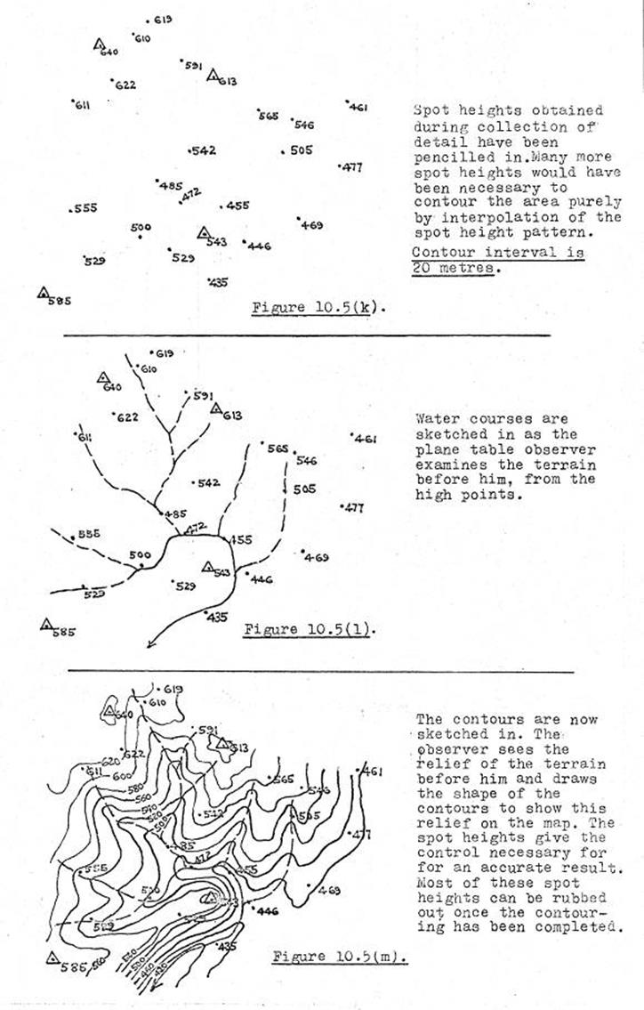
Practise is necessary, but the observer will soon start to imagine each contour line running across the country side. Image a flood in the area, gradually falling, and revealing the terrain to the observer as each contour interval is reached. See notes in the Map Reading section 10.2(e): "How to visualize relief from contours". In this case the plane table observer's task is the reverse, i.e. "How to visualize contours from relief".

The methods of contouring described are illustrated in Figures 10.5(k), (l) and (m).

The "Inaccessible Base" or "Two Point" Resection

When only two plotted control points are visible from a point whose position is required, a simple resection is impossible. The "inaccessible base" method can be used in this case. It has been included mainly for illustration of survey principles rather than for general usage, the limiting factors being the length of the base required and the distance this base is from the control points. (Draw a few diagrams with the base, one quarter the length of the distance between the control points and with varying distances between the base line and the control points. It will be seen just how weak are the angles or "cuts" which establish the trial positions of the control points).

Description of the Method:-

A & B are the plotted control points which are visible.

P is the point whose position is required.

Choose a point Q as the other end of a base, PQ. The length of this base need not be known but A & B must be visible from Q, and the base would need to be at least ¼ the length of the distance A to B.

Ignore the plotted points on the board.

A line pq is plotted at any convenient length, and A & B are intersected from P & Q which are both visited. This gives a' & b' on the board and also a figure pqb'a' which is mathematically similar to the figure PQBA in nature.

To set the board, the alidade is placed along a'b', and some object, x is sighted. The alidade is then placed along the plotted positions ab and the board is rotated until x is again sighted. Thus the board has been rotated through the error of orientation Ɵ, and is now correctly set. Erase the surplus plotting.

The correct position of p is then obtained by pulling in rays from A & B through a & b respectively.

Figures 10.5(n), (o), & (p) show the steps necessary to give the board its correct orientation and thus ready to proceed with 5 above. In these notes and in the diagrams, the capital letters, A, B, etc, refer to the positions in nature and the lower case, a, b, etc refer to the positions as plotted on the board.

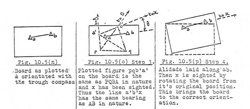
Finishing

This will depend on the requirements of any particular task; normally the minimum necessary to be shown would be the area, scale, contour interval, grid coordinates, the date and a magnetic north point.

It is important that the observer has clear instructions on all the above as well as the type of detail which must be shown and what may be omitted. For example, at some scales fences may not be shown at all, whereas at others they are a very important part of the detail. Similarly at some scales only main gates in fences, are shown, while at others it is important to show every gate.

11. Elementary Algebra, Logarithms, Plane Geometry & Trigonometry

Due to the complex formatting and possibility of error this section, despite its slightly poor quality, is presented in PDF format.

12 Survey Computations

General

The more basic of the field computations have already been dealt wlth.

These were :

Reference Marks Section 3.5

Eccentric corrections Section 3.6

Tellurometer measurements Section 4.3

In this section it is proposed to deal with other computations, some of which will be more of a background to survey work and others which will be regularly used.

12.1 Closed surveys (chain & theodolite traverses)

Bearing are specified on the Whole Circle or Azimuth method_.In this method, bearings originate from North (0^° or 360^°) and are measured clockwise from the meridian through East (90^°), South (180^°), West (270^°) and back to North.

Bearings of 0^°, 90^°, 180^°, and 270^° are known as Cardinal Bearings.

To compute the bearing of any line from the bearing of a reference line where the angle between the reference line and the required line is known the procedure is :

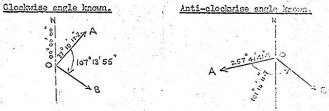
Add angle to bearing Subtract angle from bearing

Bearing 0->A = 37° 10’ 17.2” Bearing 0->A = 257° 41’ 41.8”

Clockwise angle + 107° 13’ 55.1” Clockwise angle - 101° 10’ 11.7”

Bearing 0->B = 144° 24’ 12.3” Bearing 0->B = 156° 31’ 30.1”

If the sum exceeds 360° subtract 360°. If the difference would be negative add 360° to the known bearing prior to the subtraction.

Latitude and Departures

Any line, except a cardinal line, can be resolved into two components :

A North or South component and an East or West component.

A cardinal line may only have a North or a South, or alternatively an East or a West component.

The North or South components are called Latitudes.

The East or West components are called Departures.

If there are two digits in the degrees and the figure is greater than 90°, drop the 9.

Bearing 95° 58' = 5° 58’ Direction angle.

The angles derived from these bearings is shown in the diagram, below :

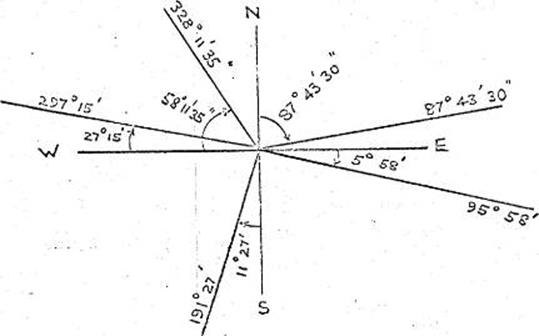
Step 2 : Multiply length of line by sine and cosine of Direction angle.

The products will be the Latitudes and Departures. But which product gives what component? Draw the following diagram :

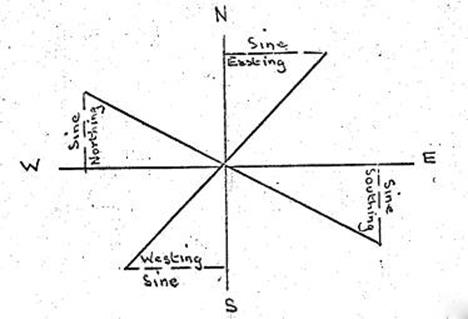
For the first few times computations are performed draw this diagram and keep it beside you. Multiply the distance by the sine first and enter the product in the component column shown by the diagram. Now that the sine component is settled in its column, and as there can only be one other component for the quadrant the product of the length and the cosine of the direction will give it.

If the length of the line and its azimuth or bearing are known, the latitudes and departures can be determined easily by the rules trigonometry pertaining to right angled triangles.

Departure or Easting = 15.215 sin 66° 15' = 13.926

Latitude or Northing = 15.215 cos 66° 15’ = 6.128

Put in other words - a point starting at 0 and travelling to A, over a distance of 15.215 metres, on a bearing of 66° 15’ would travel in an easterly direction for 13.926 metres and in a northerly direction of 6.128 metres.

Where using tables which give functions of angles from 0° to 360° :

Multiply the sin bearing by the distance to get Departure or Easting;

Multipy the cos bearing by the distance to get Latitude or Northing.

Where using tables which give functions of angles between 0° and 90° only, the following procedure is adopted.

Find the direction angle for the given bearing :

The direction angle is obtained by subtracting the cardinal bearing that is nearest in an anticlockwise direction from the bearing of the line, thus :

Bearing 125° 16’

Nearest anti-clockwise cardinal 90° 00’

Direction angle 35° 16’

Bearing 323° 11' 35”

Nearest anti-clockwise cardinal 270° 00' 00”

Direction angle 58° 11’ 35”

Another quick method :

Add the first 2 digits of 3 digit degrees together, but leave the third digit degrees and the minutes and seconds unchanged.

328° 11' 35” = 58° 11' 35° Direction angle.

If the sum of the 2 first digits gives two digits add those 2 digits together again.

297° 15' = 117° 15' = 27° 15' Direction angle.

Of course, if there are only two digits in the degrees less than 90° the figures need no alteration.

Bearing 87° 43’ 30" = 87° 43' 30” Direction angle.

Computing closed surveys (Chain & theodolite traverses)

A survey which starts at a point and is carried out by a succession of traverse lines back to the starting point is known as a "closed survey". In such a survey checks can be applied which will show the total accumulated error in the work. These total errors are known as "miscloses".

Angular Misclose

Suppose ABCDE is a closed survey. AB is the azimuth line, bearing 84° 28' 30" and at B, C, D and E the bearings of BC, CD, DE and EA are observed. If the instrument is now set up at A and the bearing AB observed it should of course read 84° 28' 30". As a matter of experience it will usually read slightly higher or lower, say 84° 29' or 84° 28'. The discrepancy so observed is called the angular misclose and is due to unavoidable errors in reading the angles.

Latitude and Departure Misclose

If a survey starts and finishes at A it is obvious that for every one metre which it advances North or East it must advance one metre South or West. To compute the latitude and departure misclose or "take out a close" the Northing or Southing (latitude) and the Easting or Westing (departure) of each line are computed and if they do not balances the discrepancy is known as the misclose. This misclose is due to errors in both chaining and observing angles.

Line				Latitudes		Departures
	Bearing	Length	North		South	East	West
AB	84° 28’ 30”	95.256	9.171			94.813
BC	172° 50’ 30”	36.600			36.315	4.516
CD	144° 29’ 30”	49.243			40.085	28.601
DE	259° 11’	61.067			11.460		59.982
EA	319° 11’	103.992	78.702				67.973
	SUM		87.873		87.860	127.975	127.955
	MISCLOSE				0.013		0.020

The misclose is shown here as two components - the misclose in the Latitudes and the misclose in the departures. It is always written under the lesser of the figures.

Now try this close for yourself by writing down the bearings and distances and computing the latitudes and departures - of course keep the example out of sight. If you get a shocking misclose in Latitudes or Departures the chances are that you have placed a latitude or departure in the wrong column. Check the positioning of the components as follows :

The directions of the components in any quadrant are the directions of the cardinal lines defining that quadrant, and the greater of the components is in the direction of the nearer of those cardinals. For example, the bearing of the fourth line is 259° 11' ie. it is between South and West and nearer to West so its components are placed accordingly, the greater in the West column and the lesser in the South column. If a line is cardinal of course it has only one component, in the direction of its bearing, and the length of that component is the length of the line.

After this check you will have reduced the misclose considerably, however, an unacceptable misclose may remain. This is probably due to :

Mistake in looking up the trig functions

Mistake in multiplication

Mistake in writing down a product.

This can be checked by repeating the whole operation, however, this is an unsatisfactory method as the same mistake may be repeated. An independent check on the multiplication can be obtained by using Gousinskys Tables.

These tables list the difference between the sine and cosine of the Direction angle.

Use them this way :

Look-up the table value for the direction angle of the line

Multiply this value by the length of the line

To the product add the lesser of the two components obtained in the close.

The sum should be within 0.001 of the value obtained previously for the larger component. If not, check the previous multiplication. In 90% of the cases you will find you have made mistakes (a), (b) or (c) above.

Now, if a mistake still remains check the addition of the components. In 1% of cases you will find a mistake.

If a misclose still remains then check the bearings and distances entered.

If after making all the checks listed above an unacceptable misclose still remained on a practical job the bearing of the misclose would be computed and the measurement of any line in the close near that bearing would be checked. However, the misclose bearing may not be anywhere near one of the traverse bearings in which case there may be mistakes in the measurement of more than one line or an angular mistake that is not apparent due to compensating blunders. Repetition of the work is required in such a case.

It is important to realise that the misclose only shows the uncompensated errors. This is particularly important in the case of chaining. It is often the practice to neglect the corrections due to temperature, sag and tension or rather to accept an approximate figure for the temperature and apply an estimated tension based on experience, which should balance the sag and tension corrections. Provided the estimated temperature is within 10° or so of the true figure and reasonable judgment is used in applying the tension the resulting errors should be well within the limits prescribed for boundary definition.

At the same time errors from these sources will tend to be uniform so that those made in Northerly or Easterly lines will tend to balance those made in Southerly or Westerly lines and the error shown by the misclose will be misleading.

Incomplete closes

The principles of computing latitudes and departures can be applied to the computation of missing bearings and distances. Computation by latitudes and departures of missing bearings and distances is usually more efficient than by solving triangles.

Case 1 : Bearing and Distance of one line missing

In the first sketch above we have an example of the information normally obtained when surveying reference marks.

A theodolite at B has determined the bearings of lines B to A and B to C and the horizontal lengths of these lines have been determined. A to C remains to be calculated.

The first step is to write the bearings down so they will be travelling in the same direction around the figure. If the bearing of A to C is required the bearings for the close must follow on in the same direction as in the second sketch above.

Bearing B to A is already given in the correct sense and remains 35^°10'. Bearing C to B is the reverse of the bearing given (B to C). To maintain the direction 180^omust be added to bearing B to C (reverse the bearing). This gives the bearing C to B of 292^o53'. The incomplete close may now be stated, the latitudes and departures computed and the "misclose” determined.

Line			Latitudes		Departures
	Bearing	Length	North	South	East	West
CB	292° 53’	7.158	2.783			6.595
BA	35° 10’	3.715	3.037		2.140
	SUM		5.820	0	2.140	6.595
	MISCLOSE			5.820	4.455

The “misclose” gives the latitude and departure of the missing line - the line required to complete the close. We now know that the missing line has a southing of 5.820 and an easting of 4.455 and consequently it must have a south easterly bearing.

In computing the missing line the lesser of the two components should be divided by the greater. The result is the tangent of the angle made with the nearest cardinal line. The direction of that cardinal is the direction of the greater component, and the side of that cardinal on which the missing line lies is given by the direction of the lesser component.

Tan θ = 4.455 / 5.820 = 0.765 464

θ = 37° 26'

The greater component is a southing so the angle computed is between the 180 cardinal and the missing line.

The lesser component is an easting so the missing line must lie to the east of the 180 cardinal.

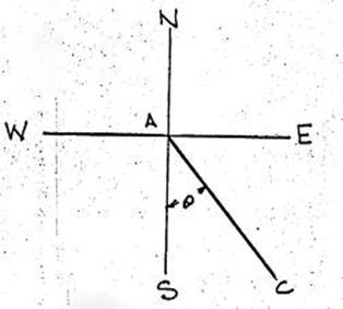
Bearing AC = 180° 00' — θ = 180° 00' – 37° 26’ = 142° 34'

The length of AC is computed by multiplying the greater component by the secant of θ.

sec 37° 46' = 1.259 349

5.820 x 1.259 349 = 7.329 = AC

The completed calculation should look like this:

Line			Latitudes		Departures
	Bearing	Length	North	South	East	West
CB	292° 53’	7.158	2.783			6.595
BA	35° 10’	3.715	3.037		2.140
	SUM		5.820	0	2.140	6.595
	MISCLOSE			(5.820)	(4.455)
AC	(142° 34’)	(7.329)		1.259349	0.765464	37° 26’

Note :

All the quantities for the computed line (bearing, length, latitude and departure) are bracketed to identify them from the quantities of the observed lines.

The computed tangent angle and secant are written in the line below the misclose.

To check the computation, three methods could be tried.

Check all latitudes and departures with Gousinsky's Tables. This method will not check the addition and subtraction of components but is usually quite sufficient.

Solve the plane triangle. Two sides and the included angle known.

Swing the bearings by a constant amount. The best way is to add or subtract an angle from the bearings so that the computed line would be cardinal.

Example Method (c)

If 37° 26' was added to the bearing of AC it would then be 180°.

Add 37° 26' to the observed bearings.

The close will now be.

Line			Latitudes		Departures
	Bearing	Length	North	South	East	West
CB	330° 19’	7.158	6.218			3.545
BA	35° 10’	3.715	1.111		3.545
	SUM		7.239	0	3.545	3.545
	MISCLOSE			(7.239)	(0.0)
AC	(180° 00’)	(7.329)

AC now computes with a bearing of 180° 00' as planned and length the same as computed previously.

All stages of the original computation have been proved by this check. However, it must be remembered that although the mathematical operations have been proved to be perfect any error that existed in the original data is thrown into the computed line.

Case 2 : Two missing distances

Suppose the lengths of AB and BC in the first close unknown. This case could arise where B is an inacessible point, or if accessible, the distances, cannot be measured.

Solution :

Alter the azimuth of the survey by adding to or subtracting from each bearing such an angle as will make the bearing of one of the incomplete lines cardinal.

In this case add 5° 31 30°. This will make AB cardinal. Compute the components of the complete lines on this altered azimuth, tabulate them as before and find the latitude and departure required to close the figure.

As one of the missing lines is cardinal it will have no latitude or departure according as it is east-west or north-south. It follows then that the latitude or departure, as the case may be, which is required to close the figure must be allocated to the other line. For this line we have its bearing and one component from which its length and the other component can be computed as sides of a right angled triangle.

These figures are inserted in the table and the departure or latitude now required to close the figure must be allocated to the remaining line, and is the length of that line.

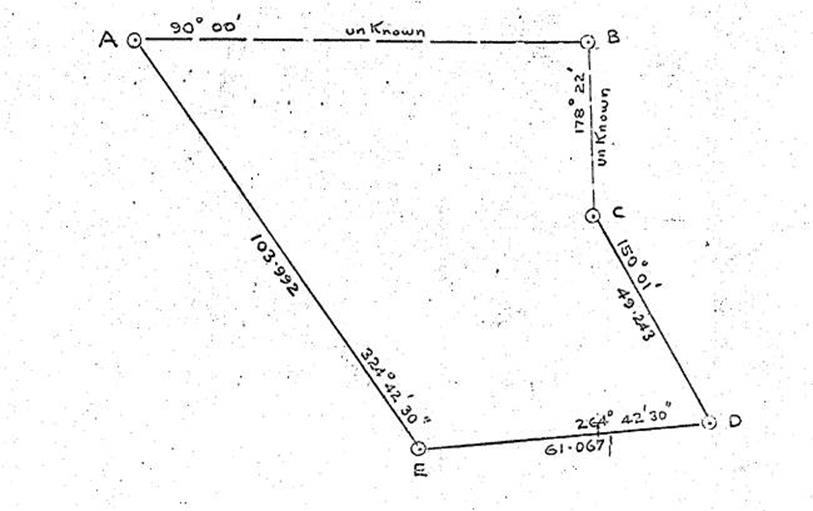
Draw a diagram approximately to scale, as above, to get a clear picture of the missing distances and the calculations required.

See next page for method of laying out the work with each step nominated.

Line				Latitudes		Departures
	Bearing	New B’rng	Length	North	South	East	West
AB	84° 28’ 30	90° 00’	95.235			95.235
BC	172° 50’ 30”	178° 22’	36.610		36.595	1.043
CD	144° 29’ 30”	150° 01’	49.243		42.653	24.609
DE	259° 11’	264° 42’ 30”	61.067		5.632		60.807
EA	319° 11’	324° 42’ 30”	103.992	84.880			60.080
				84.880	48.285	25.652	120.887
				-48.285			-25.652
				36.595			95.235

Step 1 : For BC subtract South from North to get complement (36.595) for line.

Step 2 : From South complement and bearing of line get length BC

(36.595 sec 1°38’ = 36.610) and enter in length column.

Step 3 : From length BC and bearing compute departure East (1.043).

Step 4 : Total East and subtract from West to get East for AB (95.235) and length of AB.

To check recomputed on original bearings. The figure must close or the computations are wrong.

Line			Latitudes		Departures
	Bearing	Length	North	South	East	West
AB	84° 28’ 30”	95.235	9.169		94.792
BC	172° 50’ 30”	36.610		36.325	4.562
CD	144° 29’ 30”	49.243		40.085	28.601
DE	259° 11’	61.067		11.460		59.982
EA	319° 11’	103.992	78.701			67.973
			87.870	87.870	127.955	127.955

A misclose of 0.001m would be permissible. This would occur from the errors introduced when the decimals of the components are rounded off. By computing an extra decimal place in both closes, the rounded off latitudes and departures could be made to close.

Again the assumption must be made that the measured lines have no error. Any unknown error is thrown into the computed lines.

An alternative method of solution is to find the length and bearing of the line equivalent to the known lines, as previously described. By substituting this equivalent for those known lines we obtain a triangle whose three angles are known as well as the length of one side (as so computed). This solution is to be preferred in the case of a close containing a great number of lines whose components may have already been worked out. The former method is particularly suitable when there are few lines.

Case 3 : Length of one line and bearing of another unknown

This case is solved in a similar manner to the second case. The azimuth is altered to make the bearing of the line whose length is missing, cardinal; and the computation proceeds as before until the latitudes and departures of the known lines are found, as shown :

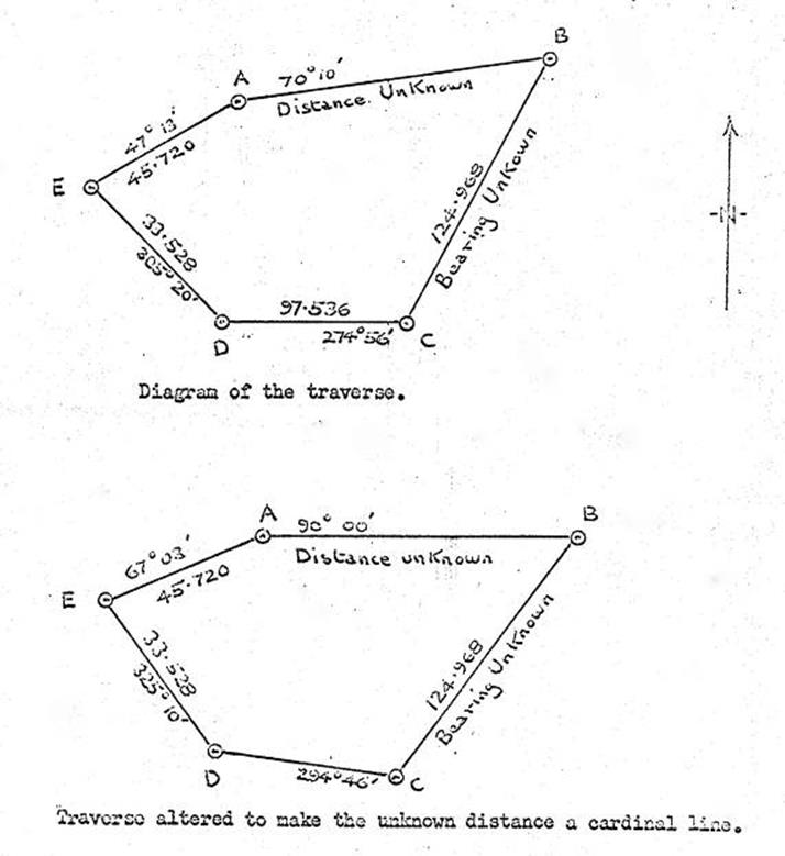
The length of the line AB, and the bearing of the line BC are required.

Line				Latitudes		Departures
	Bearing	New B’rng	Length	North	South	East	West
AB	70° 10’	90° 00’	(156.088)			(156.088)
BC	(206° 33’)	(226° 23’)	124.968		(86.208)		(90.473)
CD	274° 56’	294° 46’	97.536	40.860			88.565
DE	305° 20’	325° 10’	33.528	27.520			19.151
EA	47° 13’	67° 03’	45.720	17.828
				86.208		42.101	198.189
					(86.208)	(156.088)

The latitude of the line BC is found to be 86.203, and its length was given as 124.963. From the figure and calculation below it can be seen that two bearings could give this south latitude, i.e.,

A line 46° 23' east of the 180° cardinal line, or

A line 46° 23' west of the 180° cardinal line.

In other words an ambiguous case

In practice there should be no doubt as to which of these bearings is to be adopted. If there is, further information should be obtained such as an approximate length of the line AB, or an approximate bearing of the line BC.

From the sketch it can be seen that BC will have a south-westerly bearing. Therefore the bearing will be :

180° + 46° 23' = 226° 23'

This bearing is entered in the “New Bearing" column, and the departure for that line, computed. In this case West 90.473. The difference in departures gives the missing length.

The computed bearing is now converted to the original azimuth, and the computation is checked by closing the figure on that original azimuth. This case can also be solved by computing a closing line, AC, and solving the triangle ABC (two sides and the non-included angle.)

Case 4 : The bearings of two lines missing

In this case the solution is found by finding the bearing and length of the line equivalent to the complete lines, and solving a triangle whose sides are this line, and the two incomplete lines, to find the angles.

This case occurs in practice when two circles intersect and it is required to find the bearings of their radii from the point of intersection.

Note :

In all these cases care should be taken to avoid condtions which will give unsatisfactory results. In the second case, the solution is unsatisfactory if the lines are of nearly the same bearing when it will be found that the cosecant and cotangent of a very small angle will be involved.

The solution is similarly unsatisfactory in the third case when lines are nearly at right angles, and in the fourth case when the sum of the lengths of the incomplete lines is nearly equal to the length of the line equivalent to the balance of the traverse.

Use of Eastings and Northings instead of Latitudes and Departures

In most of the computations of rectangular co-ordinates for mapping purposes, Eastings and Northings only are used, and what has been designated as a Departure of East becomes +East, and a Departure of West becomes -East; a Latitude of North becomes +North and a Latitude of South becomes -North.

Thus, with the use of full circle bearings also, the system is very easy to grasp, and the formulae simple.

Sine bearing x distance = Diff. Easting, always.

Cos bearing x distance = Diff. Northing, always.

The signs of the DE and DN are easy to follow from this quadrant diagram :

0°

-E | +E

+N | +N

270°_______ |________ 90°

-E | +E

-N | -N

180°

The problem in 12.1(c) would appear as follows under this system :

Line
	Bearing	Length	Diff. Eastings	Diff. Northings
AB	84° 28’ 30”	95.256	94.813	9.171
BC	172° 50’ 30”	36.600	4.516	-36.315
CD	144° 29’ 30”	49.243	28.601	-40.085
DE	259° 11’	61.067	-59.982	-11.460
EA	319° 11’	103.992	-67.973	78.702
	MISCLOSE		0.020	0.013

While it is necessary to understand the use of Latitudes and Departures the simple transition to the above method should be thoroughly grasped as it will be one of the most used in mapping computations.

12.2 Spherical Excess, Closure of Triangles

In Geodetic Triangulation, the triangles or polygons may, for all practical purposes, be taken as spherical, and the sum of the angles exceeds that of the corresponding plane figure by an amount termed "spherical excess", (є).

Roughly, spherical excess is 1" for every 197 square kilometres (76 square miles).

For the terrestrial spheroid, the excess for a given area varies with the Latitude, decreasing from the Equator to the Poles. In this context the following terms should be understood :

"ρ" : The radius of Curvature in the Meridian.

Is a measure of spheroidal, or arc distance. It is used to convert linear distance along the meridian into terms of arc (Latitude differences).

"ν" : The radius of Curvature Perpendicular to the Meridian, or in the Prime Vertical.

Is a measure of spheroidal or arc distance, where such distances are at right angles to the meridian - that is, when converting Longitudes.

"ρ" and "ν" are both functions of the latitude of that place, and hence vary for different latitudes. Geodetic Tables generally give values for them in the form :

1 , 1 or 1 etc.

ρ sin 1" ν sin 1" 2ρν sin 1"

For computing spherical excess, the term 1/2ρν sin 1" is used. This is explained in 12.2.1.

12.2.1. Formulae :

Spherical Excess = Area of triangle / R² where R = radius of a sphere.

When the spheroidal shape of the Earth is used, R² becomes ρν thus in the term 1/2ρν sin 1" they are combined with sin 1" to bring the value to seconds, and ½ from the formula :

Area of a triangle = ½ab sin C.

Natural values for 1/2ρν sin 1" for all latitudes are tabulated as m x 10^-8 in the Army Map Service Tables of Latitude Functions (A.N.Spheroid).

Thus the formula becomes :

Є = ab sin C (1/2ρν sin 1")

where a & b are the two sides of the triangle, C the included angle, and 1/2ρν sin 1” is the function for the Mid-Latitude of the triangle.

12.2.2. Closing of triangles

Although the system of triangulation is now rarely used for the determining of distance there still may be some call for the closing of triangles when laying down mapping control. Also the calculation of spherical excess, the closing of triangles and reducing spherical angles to plane angles helps the understanding of many geodetic computations.

Figures :

Simple Triangles : If the observations were absolutely accurate the amount their total exceeds 180° would be the exact amount of spherical excess in the triangle.

Quadrilaterals : These yield 4 triangles as shown in Figure 12.2.2.(b). The total spherical excess in each pair of diagonally opposite triangles equals the total of the other pair. Thus immediate check of the arithmetic in totaling the observed angles and calculating the spherical excess is available.

Centre Point Triangles : The total spherical excess in the three included angles equals that of the larger triangle. Figure 12.2.2.(c).

Calculation of sides of triangles and spherical excess (Field Computation)

A good layout for the above calculation is shown in Figure 12.2.2.(d). The example is of a calculation using logarithms, but the same layout for the angular data is suitable for natural calculations, the answers just being entered in the appropriate column as they come from the machine.

Sequence for calculating the sides :

Enter observed angles and station names in their appropriate columns; lay out the work so that the known distance goes on line three, as shown. Immediately above it (on line two) enter the angle at the station opposite this known distance.

Total the observed angles in each triangle.

Arbitarily adjust the triangles to total 180° and enter these angles in the “Approx plane angle" column. Nearest second will do.

The sine formula is used and the log cosec. of the appropriate angle is used, where necessary, to make the calculation a simple addition. Fill in the logs of the angles and the known distance in the "Log Plane Angle" column.

Total lines, 1, 2 & 3, as indicated to yield one side of the triangle and 2,3, & 4 to yield the final side.

Solve all triangles in the same manner, using a calculated distance where necessary. Some distances are calculated in different triangles; in these cases minor differences in the last figures of the logs will occur.

Sequence for calculating spherical excess :

The spherical excess for each triangle is calculated twice as a check.

The Mid-Latitude for the figure is scaled from the 1:250,000 scale map.

The natural value for 1/2ρν sin 1" in this latitude, is obtained from the A.M.S.Tables. Turn this into a logarithm if the calculation is to be in that form.

Enter this figure on line one in each of the (є) Excess columns. Below these figures enter the log values for two sides and log sine of the included angle. Total each column and they should yield the same answer for the spherical excess of that triangle. Use three decimal places in the answer.

Round off the spherical excess to two places and find the misclosure of all the triangles in the figure.

Check to see that the sum of the spherical excess of the diagonally opposite triangles equals the other pair. Note that the same applies to the amount the observations exceed 180° and also the algebraic sun of the misclosure of the triangles.

12.3 Field Computation : Latitude, Longitude and Reverse Azimuth

Definitions :

Bearings and spherical angles

The difference between 2 true bearings, from any given point, is a spherical angle.

The observed angle between 2 points is a spherical angle (uncorrected for observing errors).

True bearings with approximate spheroidal distances (S) are used to calculate the Geographical Co-ordinates.

Distance S :

This is the slops distance, station mark to station mark, approximately corrected to Sea Level distance. The best available mean height for the line as taken from the map is used for the Sea Level correction, but the minor corrections for slope and Chord to Arc are disregarded.

Gauss Mid Latitude formulae :

The following formulae are satisfactory in field computations for lines of lengths likely to be met with when measuring in Australia. However, the formulae are not completely accurate for lines over 30 kilometres and are not used in the accurate office computations for lines longer than that distance.

Diff Latitude = Distance (s) cos Mid-Azimuth (Zm) / ρ sin1”

Diff Longitude = Distance (s) sin Mid-Azimuth (Zm) sec Mid-Lat / ν sin1”

Diff Azimuth (Z) = Diff Longitude x sine Mid-Latitude.

where, as defined in 12.2. ρ sin1” and ν sin1” are Radii of Curvature along the Meridian and perpendicular to the Meridian, respectively.

See attached tables and example on the Field Computation proforma.

Note that South Latitude and East Longitude are taken as being positive in this computation.

Sequence of computation :

Tabulate the Back Azimuth at the known station, add the observed angle and obtain Forward Azimuth. Tabulate Latitude and Longitude of the known station, mean altitude of known and new station, and distance between these stations. Note which quadrant the Forward Azimuth lies in and adopt the signs necessary from the sign convention panel at the bottom of the proforma.

Find the first approximate Mid Latitude using the data from the "M" Correction of Latitude Table, the Latitude of the known station, Forward Azimuth and distance to the nearest kilometre. The "M" table is listed for every 10° of Azimuth in each quadrant, using as a basis lines 10km long. For a line xkm long the correction to Latitude is found by multiplying the correction in the table by xkm/10.

To find the approximate Mid-Azimuth :

Look up the "K" factor for the approximate Mid Latitude.

Diff Z = S sine Za *K

Where : Za is the Azimuth at the known station.

K is the factor from the table.

S is the distance reduced approximately to Sea Level.

Halving the difference Z and applying, with the correct sign, to the known azimuth will give the approximate mid-Azimuth (Zm).

Computation of the Final Values :

Using Cos Zm in the Latitude formula will give Diff. Latitude and thus Latitude of the New Station. Also an accurate Mid-Latitude.

Using Sine Zm and Sec. of the accurate Mid-Latitude in the Longitude formula will give Diff. Longitude and thus the Longitude of the New Station.

Finally, this Diff. Longitude multiplied by Sine Mid-Latitude will give Diff. Azimuth, which with the Forward Azimuth,+ or - 180°, will give the Azimuth New Station to Known Station.

This result of Diff. Azimuth for lines up to 30km in these latitudes should be correct to within about 1" of the approximate result using the "K" factor.

As a final approximate graphic check, accurately plot the Known Station by Latitude and Longitude on the 1:250,000 map. Plot the position of the New Station by bearing and distance. Scale off its Latitude and Longitude; compare with the calculated values and check for gross error by the map detail.

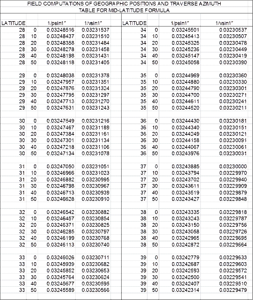
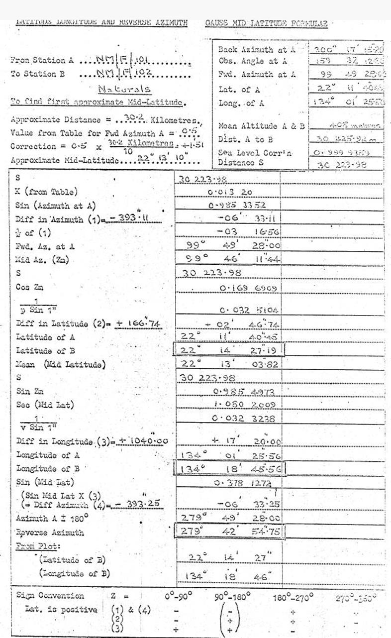
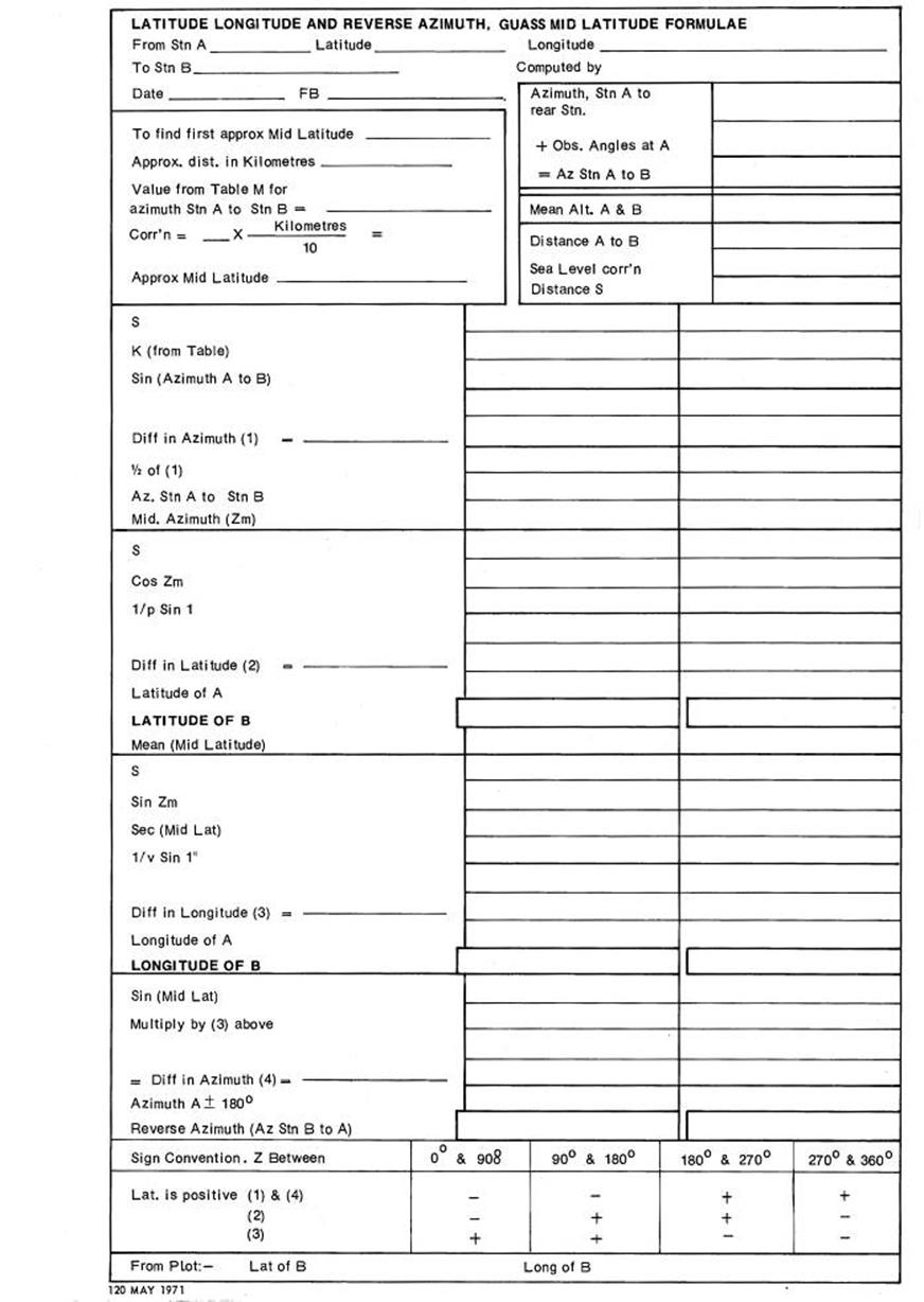
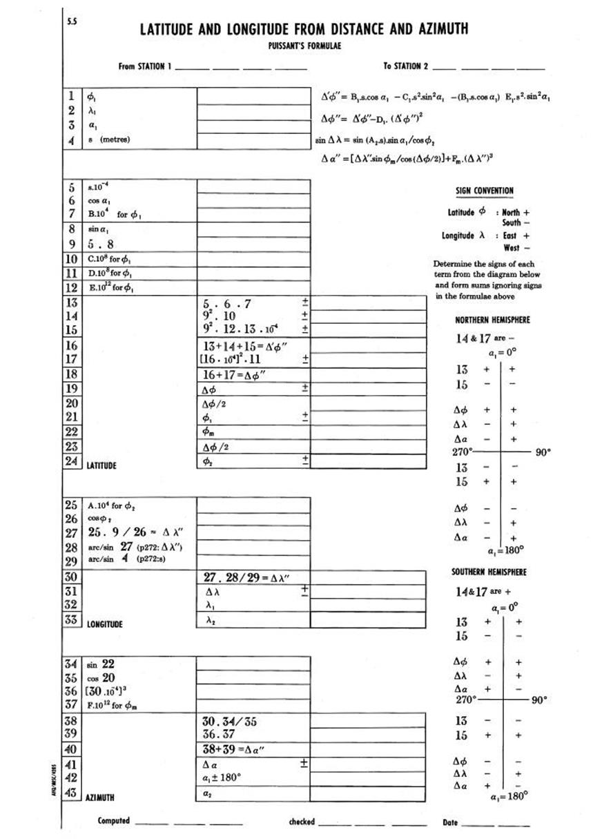
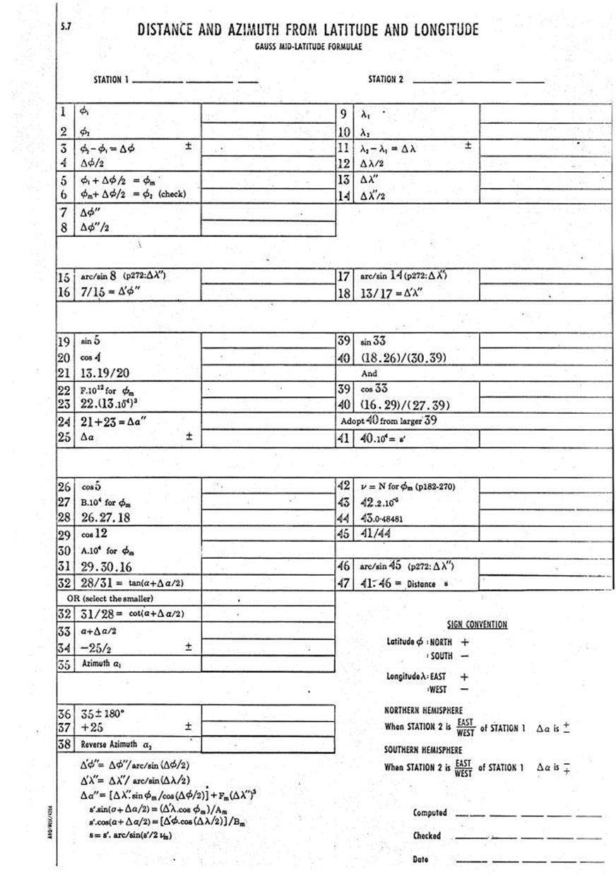
12.4 Heights from Simultaneous Reciprocal Vertical Angles

12.4.1 General

(i) Included, is a short explanation of the method of obtaining a Curvature and Refraction index from Simultaneous Reciprocal (S.R.) Vertical Angular Observations, and applying this index to a single ended vertical angle observation made immediately prior to, or following, the S.R observation.

(ii) The height of an object such as the side wall of a building can be obtained by reading a vertical angle with a theodolite, measuring the height of the axis of the instrument above ground level, and chaining the distance to the base of the wall.

Figure 12.4 shows such a simple problem:-

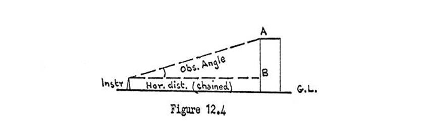
The Tan formula is used and from the diagram:-

AB = Horizontal Distance x Tan vertical angle

AB + height of instrument = Height of wall

While the above is the basis for calculating heights of intervisible Mapping Control Points along a second order, or similar, traverse, other factors prevent the problem being so simple.

(a) Curvature of the Earth

This curvature makes a distant object appear lower than it really is:-

Curvature = (Distance between the two points)² /Radius of the Earth

Thus, curvature increases proportionately to the square of the distance. The correction is always positive.

(b) Vertical Refraction

The influence of vertical refraction is not always the same, but variable, depending on air pressure, temperature, humidity, force of wind, vegetation, time of day, and even time of the year.

On a large plain the phenomenon of seeing a distant range some hundreds of miles away during unusual atmospheric conditions, is often noted soon after dawn or possibly just before dust.

The correction for refraction, can, for practical purposes be taken as always minus. Where Curvature and Refraction is used, these corrections are usually combined and the sum is practically always positive; the influence of Refraction is only about 1/7 that of Curvature.

The inability to accurately determine vertical refraction is the main difficulty in ascertaining heights by observing vertical angles. However, by observing Simultaneous Reciprocal Vertical Angles, along each line, refraction is cancelled out.

Good results can be obtained by adopting the further refinement of always observing these Simultaneous Reciprocal angles at a time of day when the air is most evenly heated (i.e., not before about 2 hours after the sun has crossed the meridian in that area, and not later than about 4 to 4½ hours after the sun crossed the meridian.

It can also be mentioned at this point, that if a non-simultaneous vertical angle were read to an unoccupied station immediately prior to, or following the simultaneous reciprocal observations a value for the Curvature and Refraction Index obtained from the S.R. observation can be used in the calculation of the non-simultaneous observation to give a fairly good result.

As shown in Figure 12.4 the height of the instrument axis is necessary to obtain the height of the wall. In actual vertical angle observations, the top of the distant hill is too indistinct to provide a clear laying mark so a target such as a heliograph, daylight lamp or beacon vanes, is always provided. Thus the correction when observing S.R. vertical angles involves two instruments and two targets along the lines shown in Figure 12.4(c).

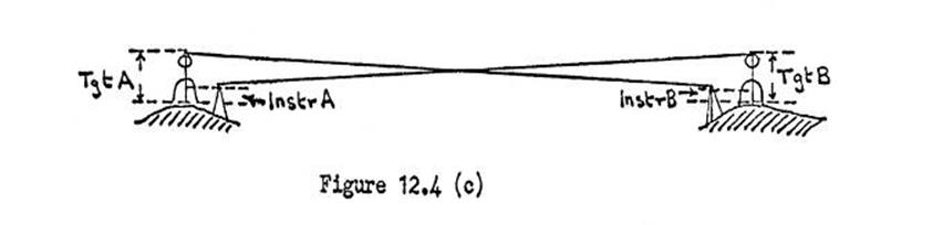
Instrument and Target Correction = (Instrument A – Instrument B + Target A – Target B) / 2

12.4.1 Computation of Heights from Simultaneous Reciprocal Vertical Angles

Formula :

Figure 12.4.1 shows 2 hills on the earth's surface, how the plumb line from each station would converge and finally meet at the centre of the earth, also how the level plane at each station would appear. This shows why vertical angles at intervisible stations are usually angles of depression.

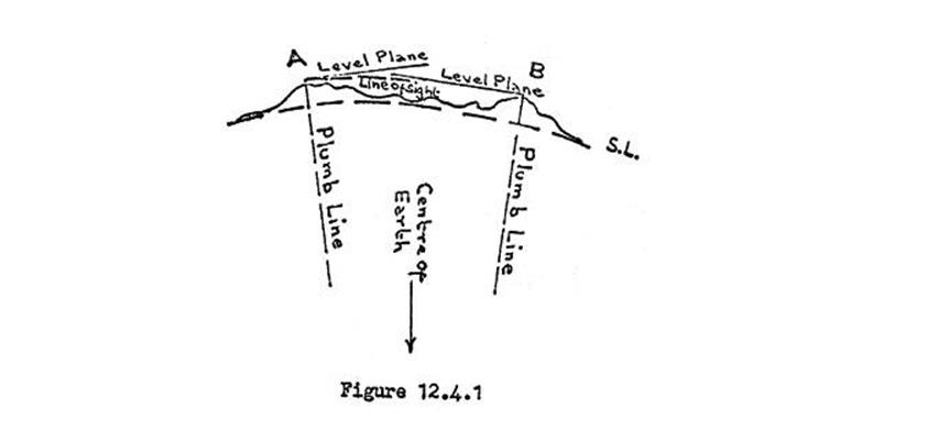
The following simplified formula, although not perfectly accurate is sufficiently so for computing most difference heights from vertical angles.

Explanations of formulae are outlined in Clarke Vol. 2 "Difference of Elevation from Reciprocal Observations."

Diff. Height = Distance between stations A & B x Tan½ (Angle at A - Angle at B) (Taking signs of observed angles into account)

In the above formula, two or the approximations are :

In the small vertical angles normally involved, the sines and tans of the angles are the same (to 6 places of logs.).

With these small angles the slope distance and horizontal distance are so similar that no inaccuracy is introduced by using the Tan and distance between stations as measured by a tellurometer.

If there is considerable difference in height between stations the problem can be resolved by:-

Using the Slope distance & sine of the vertical angle.

Compute the approximate heights using Tan; correct the slope distance to horizontal distance, then recompute the heights with this accurate horizontal distance.

Distances should not be reduced to sea level for height computations.

Components of Vertical Angular Observation

Referring again to Figure 12.4.1, and giving thought to the problem it will be realized:-

All vertical angles have an Elevation or Depression component, a Curvature component, and a Refraction component. The last two, in all the following explanations, will be combined as the "C&R" component.

If both Vertical Angles from 2 intervisible stations are of depression, the angle of least depression is made up of an elevation component (+) and a C&R component (-), and was observed from the lowest station.

The angle of most depression is made up of a depression component (-) and a C & R component (-), and was observed from the highest station.

Examine the observed vertical angles from two intervisible stations along these lines:-

Station A (Depression) 00°'11¢ 47.2" This is the Elevation angle.

Station B (Depression) 00° 14' 19.4" This is the Depression angle

From the above it can be seen that if Station A is the station of known height, the sign of the true vertical angle (when C&R are eliminated) will be Elevation, thus the difference height will be plus.

To avoid having to examine each pair of vertical angles along these lines the following can be adopted:-

At the station with the known height: Elevation angles are + & Depression angles are - i.e. signs as observed.

At the station of which ht is required: Elevation angles are - & Depression angles are + i.e. change signs.

From this:-

Station A (Known Height) Depression angle - 00° 01' 47"

Station B (Height Required) Depression angle +00° 14¢ 19²

2 ) +00° 12¢ 32²

Vertical Angle A to B +00° 06¢ 16²

It can now easily be seen how the C & R can be obtained from these figures and also the various components of both observed angles:-

Stn A to B Stn B to A

Vertical angle component (True angle) +00° 06' 16" -00° 06 16"

Curvature & Refraction component - 00° 08¢ 03² -00° 08¢ 03²

Observed vertical angle - 00° 01¢ 47² -00° 14¢ 19²

12.4.2 Sequence of Calculation using proforma (Logs or Machine)

Data Section

Enter heights of instruments and signals at each station, total and carry result to appropriate line in the calculation section.

Reciprocal Ray Section

Enter the observed vertical angles; for clarity and future checking it is a good idea to mark the elevation angles "E" and the depression angles "D" instead of + or -. Now give each angle the signs indicated; this really amounts to changing the signs of one angle as mentioned in 12.4.1, section (iii). Sum, algebraically and reduce to seconds.

Calculation.

Logs. Log the seconds, log the distance between stations. Sum of these with the constant for log tan 1² gives difference height. Apply diff. height, instrument and signal corrections to known height of the station to obtain height of distant station.

Machine. The vertical angle in seconds x distance x tan 1" = difference height. Enter the result in the appropriate column and apply with instrument and signal corrections to known height of the station to obtain height of distant station. See Figure 12.4.2 for an example computation.

12.4.3 Calculation of a Single Ray Height using C&R Index from S.R. Vertical Observation

As mentioned in 12.4(b), if a single ray vertical angle is observed to an unoccupied station immediately prior to, or following, the observation of simultaneous reciprocal vertical angles, a "C&R Index" can be calculated from the S.R. vertical angles and applied to the single ray to give fairly good results. Reasonably stable weather, and observations at the best time of the day, as previously mentioned, are necessary. Also the correct distance between the stations.

Briefly the calculation involves finding the Curvature & Refraction component of the observed angle as shown in 12.4.1, section (iii).

This value needs adjusting by the algebraic sum of the instrument and signal corrections converted to seconds. This time both instruments are plus corrections, and both signal corrections are minus corrections. The full amount of Curvature & Refraction, in seconds, is divided by the distance between stations to produce the C&R Index.

For calculating the single ray, the C&R Index x distance gives C &R in seconds, along that ray. This is applied, algebraically, to the observed angle to give the correct vertical angle between the stations. Thus, the difference height is calculated, the instrument height at the observing station and the signal height at the distant station, are the only other corrections to apply.

12.4.4 Sequence of calculation using the proforma (Logs or Machine)

Calculation of C&R Index:‑

Enter instrument and signal heights of S.R. vertical angle ray. Sum, algebraically.

Logs. The log instrument & signal correction + log cosec 1" + colog distance between stations gives instrument & signal correction; in seconds.

Machine. Instrument & signal correction (seconds) = Instrument & signal correction * cosec 1"

Distance between stations

Enter S.R. observed vertical angles; this time signs are as the angles were observed. Sum and halve to get the amount of Curvature & Refraction in the angular observation. Convert to seconds, apply instrument and signal correction to get C&R in seconds, along the line.

The C & R divided by the distance between stations gives a C&R Index.

Calculation of single ray using the C&R Index (Logs or Machine)

In the computation of height section, enter:-

Height of instrument at the observing, station, height of signal at the distant station. Sum algebraically, and enter result in the appropriate column. As one observer only, is involved, do not divide by two in this computation.

Enter the observed angle in the correct column; single ray section.

Logs. Log distance between station + log C&R Index gives Curvature & Refraction along the ray in seconds. Enter this below the observed vertical angle. The algebraic sum of these gives the vertical angle along the ray.

Machine. Distance x C&R Index gives the same result; enter, and proceed as explained in (ii), above.

Calculate the difference height, either by logs or machine in the normal manner. Apply with instrument and signal corrections to the known height of station to obtain the height of the unoccupied station.

See Figure 12.4.2, for an example computation.

12.5 Astronomical Terms met with in Observations and Computations

Altitude (h)

In the above context, the altitude can be taken as the Vertical Angle measured between the horizontal plane and the heavenly body.

Arc to Time & vice versa

Computations for Longitude are based on time, and Longitude is measured in arc. Thus, conversion of arc to time and the reverse is constantly in use. As the Earth turns once, (i.e. 360°) on its axis each 24 hours in one hour it turns 15°. Therefore divide Longitude (in arc) by 15 to get Longitude (in Time), and vice versa.

Azimuth Angle (Z)

Is the horizontal angle at the station zenith, between the celestial meridian and the great circle passing through the zenith and the star. This angle may be to the East or West of the meridian, depending on the Hour Angle (H). If the H is East, or minus, the Azimuth Angle will be on the eastern side of the meridian, and if the H is West or positive, the Azimuth Angle will be on the western side of the meridian.

Celestial Equator

The plane of the Equator extended to infinity to cut the Celestial sphere.

Celestial Poles

Points whore prolongation of the Earth's axis cuts the Celestial sphere.

Celestial Sphere

An imaginary sphere, with the Earth as centre, but at infinite distance from it, on which the “fixed stars” are imagined to be set. At various distances closer to the Earth, are the planets, sun and moon on their respective orbits.

Culmination

The crossing of the meridian by a heavenly body; i.e. the highest point above the horizon it will reach. Also called “upper transit".

Co-Latitude (c)

The complement of the Latitude; i.e. 90° - Latitude.

Co-Declination (p)

The complement of the Declination;.i.e. 90° - Declination. Also known as "Polar Distance”.

Declination (d)

The coordinate of a star which can be considered similar to the Latitude of a place on the Earth's surface. The star's Declination's are listed, in arc, North or South of the Celestial Equator. See Figure 12.5(a).

First Point of Aries (g)

An imaginary point on the Celestial Equator from which a star’s Right Ascension (RA) is measured in Time. RA is always measured from g towards the east, that is to say, in the opposite direction to that which it travels around tho Celestial Equator, because g moves with the rest of the fixed stars from East to West, i.e. clockwise.

Hour Angle (HA)

The easiest way to understand the Hour Angle is by visualizing a close circumpolar star circling the South Celestial Pole in a clockwise direction i.e., rising in the east and setting in the west. The Hour Angle, usually indicated by "t”, is the angle at the Celestial Pole between the declination circle passing through the star and the Celestial Meridian passing through the station zenith.

A star East of the station meridian has a negative hour angle equal to the period of sidereal time that it will take for the star to reach the meridian (culminate).

A star West of the meridian has a positive hour angle equal to the period of sidereal time since the star culminated.

Local Sidereal Time (LST)

When the First Point of Aries (g) is on the observer’s meridian the LST is 00 hours.

When a star is on the observer’s meridian, the LST equals that star's RA.

If it will take a sidereal hour for the star to culminate, the star's hour angle is -1hr and the LST equals RA -1hr.

An hour after the star has culminated its hour angle is +1hr and the LST equals RA +1hr.

Local Mean Time (LMT)

The instant of mean time that the sun crosses the Local Meridian.

Mean Time

Is the time kept by our clocks and is determined from a so called "mean sun". This is necessary because :

The inclination of the plane of the Equator to the plane of the Earth's orbit around the sun.

The elliptical shape of the Earth's orbit.

To provide some constant measurement of time by the sun, a "mean sun” is assumed. This is an imaginary body moving around the Celestial Equator at a uniform speed, transiting over the meridian each noon at a regular interval of time equal to the Mean Time of all the days of the year.

Nadir

A point on the Celestial Sphere directly beneath the observer; i.e. opposite to Zenith.

Sidereal Time (Star Time)

As the movement of the earth around the sun is not obvious to an observer on the earth's surface, and for the sake of simplicity, he usually imagines that the earth is fixed, and that the sun and stars revolve around the earth. Thus, the whole system of "fixed stars" appear to revolve, with absolute unity, from East to West around the earth. One complete revolution serves as a convenient unit of time for astronomical purposes. All the stars complete their circles of revolution in the same period, called the Sidereal Day. This is 3 minutes 56.56 seconds shorter than the Mean Time Day.

The datum for sidereal time is 00 hours when the First Point of Aries crosses the meridian of Greenwich. Thus Greenwich Sidereal Time (GST), at any instant, is the interval that has elapsed, measured in sidereal hours, minutes, and seconds, since the last transit of the First Point of Aries across the meridian.

Tables are available for the conversion of Mean to Sidereal Time and vice versa; also tables of Sidereal Time at 00 hours UT for each day.

Prime Vertical

Is that particular vertical circle which is at right angles to the meridian, and which therefore passes through the East-West, points of the horizon.

Right Ascension (RA)

The coordinate of a heavenly body which can be equated with the Longitude of a point on Earth, The point from which longitude originates is the meridian of Greenwich; the point from which RA originates is an imaginary point known as the First Point of Aries (g).

The RA of a star is listed in time elapsed since the First Point of Aries last crossed the meridian. See Figure 12.5(b).

Refraction

The bending of a light ray as it passes through the Earth's atmosphere. Various tables, listing corrections, are available; the altitude of the observed body, barometric pressure and temperature are required.

Sun’s Parallax

The difference between the direction of the sun, as seen from the place of observation, and as it would be seen from the centre of the earth. A correction for the Sun’s Parallax, at differing altitudes, is listed in various tables. This correction does not apply to fixed stars owing to their infinite distance from the Earth.

Universal Time (UT)

Formerly Greenwich Mean Time. Datum is 00 hours at midnight Greenwich Mean Time. Standard Times and Time Signals throughout the world and tables of sidereal time are based on this datum.

Zenith

A point on the Celestial Sphere directly above the observer. The opposite to Nadir.

Zenith Distance (z)

The vertical angle a heavenly body makes with the zenith; co-altitude, the complement of the altitude.

12.6. Time and Time Conversions, Hour Angle

General

The understanding of time is the key to understanding the movements of the stars, and the location of any selected star; also the observations for Latitude, Longitude and Azimuth. The RA of heavenly bodies are listed in time; the declination, which is the other coordinate of the stars is listed in arc; while declination is just as important in most calculations it is much easier to understand.

In astronomical observations the 24 hour clock code is always used.

Standard Time

To avoid confusion arising from the use of different local times in various towns and cities, most countries reckon their Mean Time from the mean time of a particular meridian (or meridians in large countries such as Australia). The selected meridian is an exact number of hours, or half-hours from Greenwich.

In Australia there are 3 standard meridians and thus 3 "Time Zones" (However, with the introduction of “Daylight Saving Time” in some States during the summer months there can now be many more “Time Zones” needing the observer to take special care of just what “time zone” is being used).

The three “standard time zones” are:-

Eastern 150° or 10 hours East of Greenwich

Central 142.5° or 9.5 hours East of Greenwich

Western 120° or 8 hours East of Greenwich

Time Conversions

To convert Standard Time to Local Mean Time (LMT)

Example A. Example B.

EST 11h 14m 23h 14m

Long. of Station E150° 45¢ E148° 10¢

Long. of Standard Meridian E150° 00¢ E150° 00¢

Station East of Meridian 0° 45¢ Stn. West of Meridian 01° 50¢

EST 11h 14m 23h 14m 00s

45¢ in time + 0h 03m 01° 50¢ in time - 00h 07m 20s

LMT 11h 17m 23h 06m 40s

Standard time to GMT (UT)

Subtract the longitude (in time) East of the standard meridian from standard time:-

EST 11hr 14min

East Long. of Standard Meridian 10hr 00min

GMT (UT) 01hr 14min

GMT (UT) to Greenwich Sidereal Time (GST)

A sidereal day is shorter than a mean time day by 03m 56.56secs.

A sidereal hour is shorter than a mean time hours by 00m 09.86sec. Thus to convert an interval of mean time to an interval of Sidereal Time, add, the correction (listed in Chambers Tables and the Star Almanac) to the mean time interval.

Since Midnight GMT (0hrs UT) 09h 30m have elapsed.

Convert to Sidereal Time interval 01m 34s

Sidereal interval since 0h U.T. 09h 31m 34s

+ Sidereal Time at 0hrs on 1/3/61 10h 24m 14s

GST of observation 20h 05m 48s

GST to LST

To convert the GST to LST all that is now required is to add the Longitude of the station (in time) to the GST of Observation.

GST of observation 20h 05m 48s

+ Longitude of station (in time) 08h 29m 07s (Long. 127° 16' 37.65")

28h 34m 55s
- 24h 00m 00s

LST of observation 4h 34m 55s

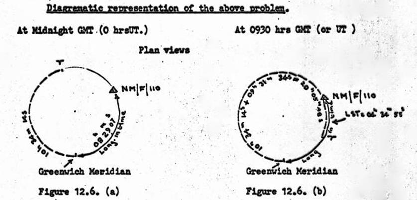
Figure 12.6(a) shows at Midnight UT on 1/3/61, the relative positions of the Greenwich Meridian, the First Point of Aries, and NM/F/110.

Figure 12.6(b) shows the path of the First Point of Aries across the meridian of NM/F/110 to a point a further 4hr 34min 55sec towards the Greenwich meridian. As shown GST is now 20h 05m 48s (i.e. this is the interval which has elapsed since g was last on the meridian of Greenwich. Thus the 04h 34m 55s which has elapsed since g was on the meridian of NM/F/110 is the LST of that point.

Determination of the Hour Angle (t)

As mentioned in the definitions, a star East of the Observer’s meridian has a negative Hour Angle. Thus its bearing will lie between 0° and 180°. Conversely a star West of that meridian has a positive Hour Angle and its bearing will lie between 180° and 360°.

When a star culminates its HA is zero and the LST is equal to the star's R.A. If a star has an HA of -1hr and RA of 10hrs the LST will be 9 hrs. Thus if we know the LST and the star's RA the HA can be determined.

Example A. Example B.

LST 9hr 11hr

RA 10hr 10hr

HA (t) - 1hr +1hr

In Example A above, the LST would be 10hr when the star culminates but as the LST is only 9hr the star must be east of the meridian and must have a negative HA.

In Example B above, the LST would be 10hr when the star culminates and as the LST is 11hr the star must have culminated 1hr previously. It is now west of the meridian and has a positive HA.

Rule to determine the Hour Angle (t)

Subtract the RA from the LST of observation. As the RA is listed in the 24hr clock mode, if the LST is too small to do this add 24 hours to the LST. This gives the H.A in the 24 hr clock mode. When computing with Shortrede's Log Tables the values at the HA, in time, can be read direct from the tables, however, when using the U.S. Dept of Commerce Natural Tables, time must be converted to arc. In both these tables values are listed for all quadrants.

12.7. Computation of Ex-Meridian Sun Observation for Azimuth

It is necessary to solve the Astronomical Triangle shown in Figures 12.7(a) and (b), the latter being in plan.

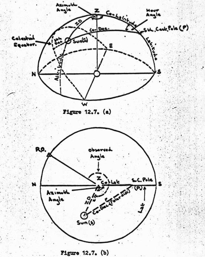
The triangle is made up of the known spherical sides:‑

Zenith Distance or Co-Altitude “z” (From field observations)

Co-Latitude “c” = 90° - Latitude. (Scaled from best available map)

Co-Declination or Polar Distance "p" - either 90° + Nth Dec. or 90° - Sth Dec. (From Star Almanac)

After field observations in which vertical and horizontal angles are read to the sun as a moving target, the problem is to calculate the Azimuth Angle PZS (known as either "Z" or "A”) to obtain the azimuth from the oblique spherical triangle PSZ, in which all sides are known in arc.

If Time is required also, the Hour Angle ZPS (known as "P") must be calculated.

Formula:-

For the calculation by Logs, use

Tan (Z/2) = 1 / (sin (s - p )) * Ö((sin (s-z) *sin (s-p) *sin (s -c)) / (sin s))

where Z is the Azimuth Angle

z is the Zenith Distance

p is the Polar Distance

c is the Co-Latitude

s = (z+p+c)/2

Computing Forms (Log and Natural Tables)

Observed ZD and UT of observations are taken from finalised Field Book.

The best available Latitude is used in the computation.

The sun's Parallax is obtained from tables on the back of the log computation form, or from Chambers Tables.

Listed in the Star Almanac, and on the back of the log computation form are tables for Mean Refraction at a standard pressure of 29.7 in. (1006Mbs) and a standard temperature of 45°F (7°C). In the Star Almanac are tables to correct the Mean Refraction Table for pressure and temperature where considered necessary.

Listed in Chambers Tables are tables for Mean Refraction at a standard pressure of 29.6 in. (1002Mbs) and a standard temperature of 50°F (10°C), also with tables to correct for pressure and temp.

Where temperature and pressures are likely to widely depart from the above, or in special cases where greater accuracy is hoped for, the required atmospheric readings should be taken immediately before and after the observation. These are not usually applied in the field check computation.

The Sun's Declination is listed in UT and at 6 hour intervals in degrees, minutes and decimals of a minute, N or S. The best method to use this table is by converting the 6 hours, and the part of the 6 hours to minutes, and take a straight proportion of the difference in declination for the six hours which should be brought to minutes and seconds instead of decimals of a minute. If available a slide rule can be used to advantage; one setting is made and all corrections read off at the same time. The multiplication by hand or machine is quite easy if no slide rule is available.

Example:-

Required, Sun's Dec. at 0822 UT on Friday 22 May, 1970.

Extracts from Dec. Table:

22 Fri. 06hrs N 20° 18.6' (20° 18¢ 30²)

Diff 3.0'

12hrs N 20° 21.6' (20° 21¢ 30²)

Thus the proportion of the 6 hours required is:

2 hr 22 min in 6 hrs of the difference, 3¢ 00"

2hr 22m * 3¢ 00² = 142m * 180² / 360m = 71² or 1¢ 11²

6hr

Thus: Tabular value for 06 hrs N 20° 18¢ 30²

Calc. value for 02hr 22min + 01¢ 11²

Value for 08hr 22min N 20° 19¢ 41²

The rest of the log calculation is a straight forward layout of the formula. Make use of the diagram to enter positions of the Sun & RO accurately enough to avoid gross error when inserting the sign of the Azimuth Angle and checking the true bearing of the RO.

In the calculation using Natural Tables the Cos formula is used:-

Cos Z = ((Sin Dec - (sine Lat * cos ZD)) / (cos Lat * sin ZD))

This formula makes a better layout for a calculation by Naturals on a proforma. Read the note on the bottom of the form to ensure that correct sign is given to Cos Z; and that the correct angle is extracted from the tables.

A way of ensuring that the correct sign for Z always eventuates for South latitudes automatically, is to reverse the sign of the declination i.e. North – negative and South – positive. As the ZD and Lat are POSITIVE the correct sign for Z will be given by the above formula.

Corrections for dislevelment of the Vertical Axis of the Theodolite

If great accuracy is to be attempted, the plate bubble should be read at each pointing on the sun. Procedure is the same as laid down for the observation for Azimuth on Sigma Octantis in section 3.8; notes on ascertaining the sign of the bubble correction and calculating it are in section 12.8.

Examples of Sun Azimuth computations.

These are shown in Figure 12.7(c) Log computation.

12.8. Computation of Azimuth from a close Circumpolar Star - Log or Natural Tables

The usual close circumpolar star used for the determination of azimuth in Australia is Sigma Octantis. With a declination of approximately 89° 04'S and its fastest movement in azimuth (at upper or lower transit) being only some 17 seconds of arc in 1 minute of time makes pointing easy, and a time accuracy of 0.5 seconds is all that is normally required.

Figure 12.8(a) illustrates this slow movement

Movement of Sigma Octantis at various Hour Angles, Latitude 30°.

One quadrant only shown.

The field book is reduced as described in Section 3.8; the meaned time of each round reduced to UT, and the mean of each round of horizontal angles is required, also the vertical angle (nearest minute) and bubble reading.

The Hour Angle of each pair of observations are calculated on the proforma and the corresponding horizontal and vertical angles entered in their appropriate spaces.

The problem is to calculate the Azimuth Angle which the star made with the true meridian at each of the hour angles. This angle may be to the East or West of the meridian depending on the hour angle. Using the 24 hour clock code in all steps from the initial recording of the mean time of the observation to the conversion of the HA to arc, the, decision as to the quadrant in which the star lies at the time of the observation is quite simple.

It must not be forgotten that the requirement for this azimuth computation is a knowledge of the accurate Latitude and Longitude of the position from which the observations were made.

Formula :

In solving the spherical triangle ZPS (Figure 12.8.(b) this time, the accurately known values are:-

The side ZP (Co-Lat)

The side PS (Co-Dec. or Polar Distance "p")

The included angle ZPS (Hour Angle "t")

The formula used for the Log calculation is:‑

A" = sec f * p" * sin t + (p")² sin t * cos t * tan f * sin 1"

Where :

A" = Azimuth Angle in seconds or arc

p" = Polar Distance in seconds of arc

t = Hour Angle

f = Latitude

That part of the equation, (p")² sin t * cos t * tan f * sin 1", gives the small correction for the sign of the sin and does not need solving, the values being tabulated in Albrechts Tables for ±Log(1/1-a). Where the star is above elongation the correction is plus, and where the star is below elongation the correction is minus.

There is a proforma for Natural Tables using the above formula; however the more straight forward formula and the one in general use within the Division is:‑

A" = ((206264.8 *sine t) / (a-(b * cos t)))

Where :

a = sin f and

b = (sin dec * cos f / cos dec)

A proforma is available for this formula and all these proformae are straight forward as long as the signs of the angles in their various quadrants are watched carefully. Shortrede’s Log Tables show this clearly as do the 8 figure U.S. Dept of Commerce Sine & Cosine Natural Tables. The Secant can be obtained by 1/cos and the Tan Dec (nearest Minute) from Chambers Tables.

Determination of Azimuth from the Azimuth Angle

The proforma probably makes this explanation redundant, however the understanding of the problem is important in case computations have to be done when no proforma is available.

As the azimuth of the meridian from the station to the South Pole is 180°, and the computation has been to find the angle that the star made with this meridian (azimuth angle), the star’s azimuth is obtained by :

Subtracting the azimuth angle from 180° if the star is East of the meridian, or adding the azimuth angle to 180° if the star is West of the meridian.

Once the azimuth to the star has been computed, the azimuth to the R.O. can be determined by applying the horizontal angle. As the clockwise angle from the R.O. to the star is always observed, the azimuth to the R.O. is arrived at by subtracting the horizontal angle from the azimuth of the star. If the azimuth of the star is less than the horizontal angle, add 360° to the azimuth of the star, before subtraction.

180° 00' 00"

Azimuth angle - 40’ 25.2

Azimuth or Sigma Octantis 179 19 34.8

Add 360° 360 00 00

539 19' 34.8

Subtract angle RO to Star 262 05 51.4

Azimuth to RO 272 13 42.4

Note :

Sketch not to scale, Azimuth angle has been exaggerated.

Figure 12.8. (c) Determination of azimuth from azimuth angle.

Time curvature correction

Where undue delay between FL & FR pointings on the star has been caused by cloud, etc., a correction is necessary. Figure 12.8.(d) gives a table for this correction, the formula is from Bomford's "Geodesy". In general practise, however, it has been found better to discard such pointings in the field and observe additional rounds to take their place.

Figure 12.8.(d)

Plate bubble corrections to astronomical observations for azimuth

The first principle to get clearly in mind is that the azimuth of the star, as calculated is correct, and dislevelment of the theodolite as shown by the plate bubble bears no part in this result as it was calculated from accurate Time, Latitude, Longitude and the astronomical co-ordinates, of the star.

The second principle is that the bubble correction for dislevelment is applied to the horizontal angle, R.O. to star.

The correction to the horizontal angle is :

If readings are high (+), to the left, the instrument is tilted to the right, therefore the instrument read a horizontal angle which was too small, thus the correction must be added to the observed angle. See Figure 12.8.(e).

If readings are high (+) to the right, the instrument is tilted to the left, therefore it read a horizontal angle which was too large and the correction must be subtracted from the observed angle. See Fig. 12.8.(f).

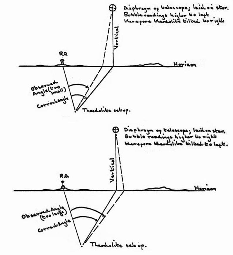
Figures 12.8.(e) and 12.8.(f).

The bubble is read from the centre outwards; the values being estimated to 0.1 of a division. They are recorded Left & Right, as seen from the stance of the observer. In the case of a close circumpolar star, in the Southern Hemisphere, the field books show East for Left and West for Right. The layout of the plate bubble of the Wild Theodolites and suggested method of reading them, is :

Plate Bubble Wild T2, Plate Bubble Wild T3.

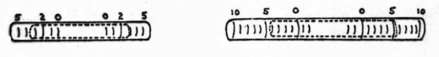
+L 3.7 -R 2.9 + L 4.2 - R 5.3

1 Div. = approx 20" 1 Div. = approx 6.5"

To calculate the bubble correction in divisions and decimals

(Sum L - Sum R)/n = correction, where n is the number of ends read.

To calculate the bubble correction in seconds of arc

Tan Alt x bubble corr'n (in Divs & decimals) x value 1 Div of bubble = Correction

Example

L. R.

5.0 5.6 Altitude 29° 57’

5.0 5.6 1 Div = 6.5”

4.7 5.3

4.6 5.4

+19.3 -21.9

+19.3

-2.6 -2.6/8 (ends) = -0.32

Bubble Corr'n = Tan (29° 57’) * (-0.32) * (6.5”) = -01.20"

Observed Horizontal angle 271° 49’ 36.2”

Bubble correction -01.2"

Corrected Horizontal angle 271° 49’ 35.0”

True bearing star 178° 56’ 47.6” (add 360°)

- Corrected Horizontal angle 271° 49’ 35.0”

True bearing R.O. 267° 07’ 12.6”

Special Note :

When using the proforma for observations on close circumpolar stars, to avoid the extra step of correcting the horizontal angle before subtracting it from the true bearing of the star, the signs printed on the form for the calculation of the bubble correction have been reversed, so that the correct true bearing is obtained by just applying the correction straight to the uncorrected bearing of the R.O. Also, as previously mentioned, Left is listed as East, and Right as West.

The above example as it would appear on the Proforma :

Example

E W

5.0 5.6 Altitude 29° 57’

5.0 5.6 1 Div = 6.5”

4.7 5.3

4.6 5.4

-19.3 +21.9

-19.3

+2.6 +2.6/8 (ends) = +0.32

Bubble Corr'n = Tan (29° 57’) * (+0.32) * (6.5”) = +01.20"

True bearing star 178° 56’ 47.6” (add 360°)

Observed Horizontal angle 271° 49’ 36.2”

Uncorrected bearing R.O. 267° 07’ 11.4”
Bubble correction +01.2"

True bearing R.O. 267° 07’ 12.6”

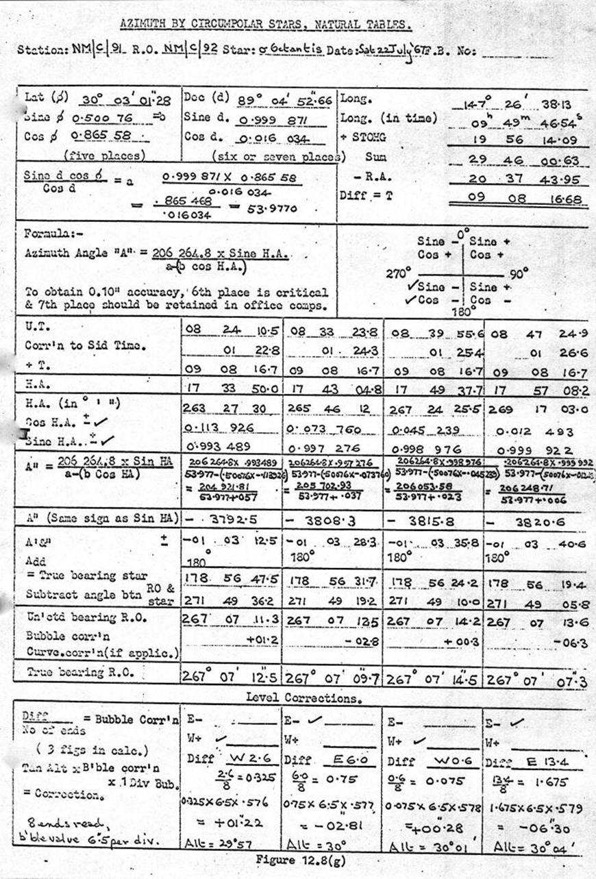
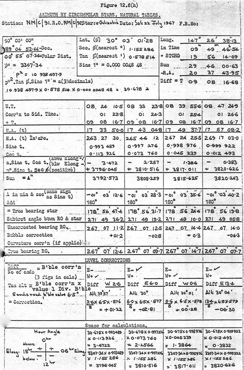
Interpolation of the R.A. & Declination of Sigma Octantis

From the Star Almanac

A table is given showing the apparent position of Sigma Octantis for every tenth Upper Transit at Greenwich. Positions are given to the nearest second of Time in R.A., and the nearest second of Arc in Declination.

For the accuracy required in the field computation, and taking into account the accuracy of the table, a direct interpolation to the day of observation is sufficient.

From the FK4

A table is given showing the apparent position of Sigma Octantis for every Upper Transit at Greenwich. Positions are given to two decimals of a second of time in R.A., and to two decimals of a second of arc, in Declination.

For the field computation, the values tabulated for the time of Upper Transit at Greenwich, are sufficiently accurate without interpolation. In the extreme case the error in the field computation will only be about 0.5", in the computed azimuth.

If very accurate results are required, it is necessary to ascertain the U.T. of Upper Transit on the day of observation, and interpolate between this and the U.T. of the observation. This is not quite straightforward; depending on the Sidereal Time at 0hrs U.T. and the R.A. of Sigma Octantis, the interpolation may be forward towards the next day, or backwards towards the previous day’s value.

The following examples illustrate the problem :

Example 1 : Where Siderial Time at 0hrs U.T. is less than R.A.

Date of Observation, 17 Jan 1971.

U.T. of Observation (approx mean time of whole observation) 14h 24m

U.T. of Observation (in days and decimals of a day) 17.60d

R.A. of Sigma Octantis same date (nearest minute here) 20h 39m

Where R.A. is less than Siderial Time add 24 hrs.

- Siderial Time at 0hrs U.T. same date 7h 43m

U.T. of Upper Transit Sigma Octantis 17 Jan 12h 56m

U.T. of Upper Transit (in days & decimals) 17.54d

Thus the tabulated value in the FK4 for the Upper Transit of Sigma Octantis is for the 17.54 day of Jan, 1971. The observation was done at 17.60, therefore the amount of interpolation is for 0.06 of a day from the tabulated time of Upper Transit on 17^th towards that of the 18^th.

FK4 value on 17 Jan. RA 20h 39m 20.65s Dec. -89° 04’ 13.08”

FK4 value on 18 Jan 20 39 20.49 -89° 04’ 12.72”

0.16 0.36

0.06 x 0.16 = 0.010 0.06 x 0.36 = 0.022

FK4 values 17th RA 20 39 20.65 Dec. -89 04 13.08

Corrections -.01 - .02

Values at time of Obs 20 39 20.64 -89 04 13.06

Figures 12.8 (i) and (j) illustrate the above problem.

At 0hrs U.T. 17 January 1971. Figure 12.8.(i) shows the positions of g and Sigma Octantis. It can be seen that Sigma Octantis will reach Upper Transit at about 13hrs on the 17th (i.e. in days & decimals, 17.54).

At 14h 24m U.T. same day (Time of Observation). In Figure 12.8.(j) it can be seen that Sigma Octantis has recently crossed the Greenwich Meridian,(i.e. Upper Transit when its values are tabulated). Thus the interpolation must be forward from the tabulated value of that day by about 1.5hrs, or 0.06 of a day.

Example 2 : Where Siderial Time at 0hrs U.T. is greater than R.A.

Date of Observation, 18 Sept 1971.

U.T. of Observation (approx mean time of whole observation) 09h 08m

U.T. of Observation (in days and decimals of a day) 18.38d

R.A. of Sigma Octantis same date (nearest minute here) 20h 42m

Where R.A. is less than Siderial Time add 24 hrs.

- Siderial Time at 0hrs U.T. same date 23h 45m

U.T. of Upper Transit Sigma Octantis 18 Sept 20h 57m

U.T. of Upper Transit (in days & decimals) 18.87d

Thus the tabulated value in the FK4 is for the 18.87 day of Sept, 1971. The observation was done at 18.38, therefore the amount of interpolation is for 0.49 of a day from the tabulated time of Upper Transit on 18^th backwards to that of the 17^th.

FK4 value on 18 Sept RA 20h 42m 21.19s Dec. -89° 04’ 11.21”

FK4 value on 17 Sept 20 42 22.13 -89° 04’ 10.95”

0.94 0.26

0.49 x 0.94 = 0.461 0.49 x 0.26 = 0.127

FK4 values 18th RA 20 42 21.19 Dec. -89 04 11.21

Corrections +.46 - .13

Values at time of Obs 20 42 21.65 -89 04 11.08

Figures 12.8 (k) and (l) illustrate the above problem.

At 0hrs U.T. 18 Sept. 1971. Figure 12.8.(k) shows the positions of g and Sigma Octantis. It can be seen that Sigma Octantis will reach Upper Transit at about 21hrs U.T. on the 18^th (i.e., actually in days & decimals, 18.87).

At 09h 08m same day (Time of Observation). In Figure 12.8.(l) it can be seen that Sigma Octantis has still a long way to go to reach Upper Transit. Thus the interpolation must be backwards from the tabulated values of the date of observation, towards the previous days' values. The amount is about 12 hours, i.e. about 0.50 days.

Example 3 : On the date of the Double Upper Transit

Date of Observation, 2 Aug 1971.

U.T. of Observation (approx mean time of whole observation) 09h 36m

U.T. of Observation (in days and decimals of a day) 02.40d

R.A. of Sigma Octantis same date (1^st Upper Transit) 20h 42m 37.33s

- Siderial Time at 0hrs U.T. same date 20h 39m 44.86s

U.T. of Upper Transit Sigma Octantis 2 Aug 02m 52.47s

U.T. of 1^st Upper Transit (in days & decimals) 02.002d

R.A. of Sigma Octantis same date (2^nd Upper Transit) 20h 42m 37.60s (+24hrs)

- Siderial Time at 0hrs U.T. next day 20h 43m 41.42s

U.T. of 2^nd Upper Transit Sigma Octantis 2 Aug 23h 58m 56.18s

U.T. of 2^nd Upper Transit (in days & decimals) 02.999d

Thus it can be seen that the interpolation can be taken forward from the First Upper Transit, or backwards from the second Upper Transit. In this example, the interpolation is taken forward from the First Upper Transit.

Time and date of observation 02.400
U.T. of 1st Upper Transit 02.002

00.398

Thus the interpolation is 0.398 forward from the 1st Upper transit towards the 2nd Upper Transit.

FK4 value 24 Aug (1^st Upper Transit) RA 20h 42m 37.33s Dec. -89° 03’ 58.02”

FK4 value 24 Aug (2^nd Upper transit) RA 20 42 37.60 -89° 03’ 58.27”

0.27 0.25

0.398 x 0.27 = 0.107 0.398 x 0.25 = 0.099

FK4 values 1^st Upper Transit 20h 42m 37.33s Dec. -89° 03’ 58.02”

Corrections +.11 +.10

Values at time of Obs 20h 42m 37.44s -89° 03’ 58.12”

Formula for all above cases :

n (#) = Y - Z

where :

n is the decimal of a day for which interpolation is required.

Y is the decimal of a day for the time of observation.

Z is the RA of Sigma Octantis for the day of observation minus Siderial Time at 0hrs U.T. same day (converted to decimals of a day).

(#) If n is positive, interpolate forward from the day of observation to the next day.

If n is negative, interpolate backwards from the entries for the day of observation towards the previous day.

Time curvature correction.

This is only rarely needed in computing Sigma Octantis azimuth observations. The correction is necessary if there is a long time deiay between the FL and

FR pointings on the star. Once the observer is experienced, this time delay would not be worth taking into account, and would only occur under cloudy conditions. However, under such conditions, it is advisable that once the time delay reaches about 7 minutes without the star re-appearing, that arc be abandoned and a fresh start made from the RO when the sky has cleared.

Figure 12.8.(d) gives a time correction table. It is compiled from the formula in Bomford's "Geodesy", Page 257.

12.9 Barometric Heighting with Mechanism Barometers – Field Computation

12.9.1 Figure 12.9(a) shows in general terms what is involved in calculating difference heights by comparative Barometric readings and is enlarged upon in the following notes.

Step 1. Base & Remote Baro's read simultaneously at Base before the Remote is taken to the Remote Station.

Step 2. Base &Remote Baro’s read each hour, on the hour while the instruments are apart.

Step 3. Base & Remote Baro' s read simultaneously at Base immediately the Remote returns from the Remote Station

______^___________ -------------------------

Base (at BM) While Baro's are being read during the day it is assumed that the pressure at this point is the same as at the Base. ^

Difference between Base readings and Remote readings |

(after allowing for instrument comparison) gives |

difference in height in millibars. |

_______________________^______

Remote

Figure 12.9(a).

Field Book

The page in the field book has been designed so that no transcription to data sheets for programming is required, a photocopy of the field book page being sufficient. Thus it is important that all entries are clearly and neatly written in the correct space.

The Base Barometer readings are transcribed from the Base Barometer book on return from the Remote station. This transcription should be checked by a second person, as these transcribed readings are those which will be used in the computations.

Normally, while the instruments are apart, all readings will be taken on the even hour, however if this has not been the case, the Base readings must be taken from the graph at the same instant of time as the Remote readings. It is normal practise to draw a graph of both Base & Remote station readings. If the curves are not generally parallel, unsuitable weather conditions, or errors in reading the barometers are indicated and unreliable heights can be expected. Generally two instruments are used at each position.

Details of the Computation.

The computation is a simple one and the accuracy of the results rely on the comparatively stable weather conditions generally covering inland Australia. Thus all that is involved is :

(i) The simultaneous comparison of Base and Remote Barometers immediately before leaving for, and after returning from, the Remote Station; this enables the Base instruments pressure readings, while the instruments were apart to be adjusted to the same scale value as the Remote instruments. Temperatures taken at each station, at the time of all readings are also necessary.

(ii) The difference between the "adjusted pressure" at the Base, (i.e., the mean of all the readings at the Base while the instruments were apart, plus or minus the "adjustment") and the mean of all the readings at the Remote Station, (i.e., Mean Remote Pressure) gives the difference height in pressure, in millibars. This is converted to feet/metres to give the difference height between the stations.

(iii) As the value of the millibar in feet varies with the temperature of the column of air and the height above sea level, the pressure at the mid height between stations, and the mean of the temperature road at the stations, is required in the calculation. Thus the difference height in feet is calculated as a simple proportion from the difference height in pressure, allowing for the mean temperature.

Steps to be followed in the computation :

1. Comparison of simultaneous Base and Remote readings (taken before and after visiting the Remote Station).

The difference is found between these means of Base and Remote instruments. This difference is the amount needed to "adjust" to the same scale, the Remote and Base instruments. Note that the Base is "adjusted" to agree with the Remote. This completes the "Comparison of Instruments", section of the computation.

2. Calculation of Difference Height (in pressure)

The "adjustment" is now applied to the mean of all the Base readings taken while, the instruments were apart, i.e., while the Remote instruments were at the Remote Station. The difference between the adjusted pressure at the Base and the mean pressure of all the readings at the Remote Station gives the Difference Height in pressure.

3. Temperature Correction

The Mean Temperature in °C + 273 = Temperature Absolute.

Temperature Absolute x 95.977 = K, which gives the value of the millibar at that temperature at sea level.

Tables to °C are available for these K factors.

4. Calculation of the Difference Height in feet from the Difference Height in pressure

Difference Height in pressure

Mid. Height in pressure x K gives Diff. Height in feet

(taking into account the mean temperature)

Finalising the Calculation

The Base is normally established at a BM, or close enough to enable a Level connection to be made to the BM. The difference height between the Base and the Remote Station obtained by the Barometric Heighting, is applied to the reduced level of the Base Station to give the height of the Remote Station, in feet; convert to metres if necessary.

Examples of Field Notes and the Calculation of the Remote Station height

Figure 12.9(b) shows a field book page showing entries taken at the Remote Station and the simultaneous entries transcribed from the Base Barometer Book.

Figure 12.9(c) shows a graph of the Baro readings at the Base and Remote Stations. All instruments are graphed separately.

Figure 12.9(d) illustrates a height calculation on the most simple of proforma for field use.

Figure 12.9(e) illustrates the same calculation on a more complicated form which takes into account a time differential when calculating the adjustment to be applied to the Base readings. However, practise has shown this correction is not warranted in field calculations, as any variation to the amount of the adjustment is negligible. i.e., Nil to 0.05 Millibars.

Figure 12.9(f) shows a Table of Corrections for K, where:

K= 95.977 *(°C + 273) from above for answer in feet or

K= 29.25 * C +273) for answer in metres.

"K" FACTOR FOR TEMPERATURE CORRECTION
*K = 95.977 (°C + 273) for feet or 29.25 (°C + 273) for metres*

Deg C	K (ft)	K (m)	Deg C	K (ft)	K (m)	Deg C	K (ft)	K (m)	Deg C	K (ft)	K (m)
0	26202	7985	12	27353	8336	24	28505	8687	36	29657	9038
0.5	26250	8000	12.5	27401	8351	24.5	28553	8702	36.5	29705	9053
1	26298	8015	13	27449	8366	25	28601	8717	37	29753	9068
1.5	26346	8029	13.5	27497	8380	25.5	28649	8731	37.5	29801	9082
2	26394	8044	14	27545	8395	26	28697	8746	38	29849	9097
2.5	26442	8058	14.5	27593	8409	26.5	28745	8760	38.5	29897	9111
3	26490	8073	15	27641	8424	27	28793	8775	39	29945	9126
3.5	26538	8088	15.5	27689	8439	27.5	28841	8790	39.5	29993	9141
4	26586	8102	16	27737	8453	28	28889	8804	40	30041	9155
4.5	26634	8117	16.5	27785	8468	28.5	28937	8819	40.5	30089	9170
5	26682	8132	17	27833	8483	29	28985	8834	41	30137	9185
5.5	26730	8146	17.5	27881	8497	29.5	29033	8848	41.5	30185	9199
6	26778	8161	18	27929	8512	30	29081	8863	42	30233	9214
6.5	26826	8175	18.5	27977	8526	30.5	29129	8877	42.5	30281	9228
7	26874	8190	19	28025	8541	31	29177	8892	43	30329	9243
7.5	26922	8205	19.5	28073	8556	31.5	29225	8907	43.5	30377	9258
8	26970	8219	20	28121	8570	32	29273	8921	44	30425	9272
8.5	27018	8234	20.5	28169	8585	32.5	29321	8936	44.5	30473	9287
9	27066	8249	21	28217	8600	33	29369	8951	45	30521	9302
9.5	27114	8263	21.5	28265	8614	33.5	29417	8965	45.5	30569	9316
10	27161	8278	22	28313	8629	34	29465	8980	46	30617	9331
10.5	27209	8292	22.5	28361	8643	34.5	29513	8994	46.5	30665	9345
11	27257	8307	23	28409	8658	35	29561	9009	47	30713	9360
11.5	27305	8322	23.5	28457	8673	35.5	29609	9024	47.5	30761	9375

Figure 12.9(f).

12.9.2 Alternative formula for computation by logs

For general interest, rather than for field use, the following notes have been compiled from a paper by Lt-Col. C.A.Biddle, R.E., Senior Lecturer in Surveying, University College, London.

“If simultaneous readings of pressure have been obtained at two points, a & b, the text book relation connecting their height difference (hb - ha) with pressure readings pa and pb, is usually given in the form:-

hb - ha = { c *(Log (Pa / Pb)) * (Tm / Ts) } * (1+x)(1+y) where:

c is some constant

Tm is the absolute mean temperature of the air column between a & b

Ts is the standard temperature

x is a small correction for the humidity of the air column

y is a very small correction for the change in gravity with Latitude.

This formula can be considerably simplified.

Since Ts is a constant, we can write (c/Ts) = K, also, an increase in humidity has a similar effect to an increase in Tm. Instead of using the separate multiplying factor (1+x) for a humidity correction, we may add to Tm the small temperature correction Th which would have the same effect. Similarly, we may replace the gravity change factor (1+y) by adjusting the temperature again by the correction for Ti of equivalent effect. The adjusted temperature Tm + Th + Ti may then be known as the virtual temperature, Tv; it is the temperature of the air column of zero humidity at standard Latitude which would exert the same pressure as the actual column of temperature Tm. For most purposes the humidity and Latitude corrections may be neglected altogether; the former will be insignificant at low temperatures, the latter in Latitudes between 30° and 60°.

The formula thus reduces to:-

(hb – ha) = KTv (log(pa/pb))

Since log tables are required for one term above, it will be most convenient to complete the computation by logs.

log (hb – ha) = log (KTv) + log(log pa – log pb)

A table of log KTv, to give height difference in feet is at the end of this extract to five figures. This is sufficient as it will not be worthwhile giving final height differences more accurately than to the nearest foot”. Note KTv is also given to aid computation by machine.

Example of height computation using the above Log formula

Calculation for feet metres

Pressure at Remote pa 963.78 Log = 2.983 98 = 2.983 98

Adjusted pressure at Base pb 962.02 Log = 2.983 18 = 2.983 18

Diff = 0.000 80 = 0.000 80

Log Diff = 4.903 09 = 4.903 09

Tabular value for KTv(24°C)= 4.817 54 = 4.301 56

1.720 63= 1.204 65

Diff height = -52.6ft = -16.02m

Check 52.6 x 0.3048 = 16.03m

which also agrees with the previous calculations.

In the above log calculation, once the difference between log pa and log pb has been obtained, the balance of the calculation may be done by machine if the difference log pa - log pb is left in log form, thus:-

Diff. x Temperature Absolute °C x 221.266 = difference height in feet, where 221.266 (67,442 metres) is the constant given in the Smithsonian Meteorological Tables, 1958 edition page 203, for use with the log formula.

The above example, using a machine, reverts to:

0.00080 * (24 +273) * 221.266 = 52.57 ft or 16.02m.

Or taking KTv from the Table 0.00080 * 65696 = 52.56 ft or 0.00080 * 20024 = 16.02 m.

TABLE OF TEMPERATURE CONSTANT TO GIVE HEIGHT IN FEET - LOG COMPUTATION
*Log KTv = log (221.2 (°C + 273))**
Deg C	K	Deg C	K	Deg C	K	Deg C	K
0	4.78095	12	4.79963	24	4.81754	36	4.83474
0.5	4.78174	12.5	4.80039	24.5	4.81827	36.5	4.83545
1	4.78254	13	4.80115	25	4.81900	37	4.83615
1.5	4.78333	13.5	4.80191	25.5	4.81973	37.5	4.83685
2	4.78412	14	4.80267	26	4.82046	38	4.83755
2.5	4.78491	14.5	4.80342	26.5	4.82118	38.5	4.83824
3	4.78569	15	4.80418	27	4.82191	39	4.83894
3.5	4.78648	15.5	4.80493	27.5	4.82263	39.5	4.83964
4	4.78726	16	4.80568	28	4.82335	40	4.84033
4.5	4.78805	16.5	4.80643	28.5	4.82407	40.5	4.84102
5	4.78883	17	4.80718	29	4.82479	41	4.84171
5.5	4.78961	17.5	4.80793	29.5	4.82551	41.5	4.84241
6	4.79039	18	4.80868	30	4.82623	42	4.84310
6.5	4.79117	18.5	4.80942	30.5	4.82694	42.5	4.84378
7	4.79194	19	4.81017	31	4.82766	43	4.84447
7.5	4.79272	19.5	4.81091	31.5	4.82837	43.5	4.84516
8	4.79349	20	4.81165	32	4.82908	44	4.84584
8.5	4.79426	20.5	4.81239	32.5	4.82980	44.5	4.84653
9	4.79503	21	4.81313	33	4.83051	45	4.84721
9.5	4.79580	21.5	4.81387	33.5	4.83122	45.5	4.84789
10	4.79657	22	4.81461	34	4.83192	46	4.84858
10.5	4.79734	22.5	4.81534	34.5	4.83263	46.5	4.84926
11	4.79810	23	4.81608	35	4.83334	47	4.84994
11.5	4.79887	23.5	4.81681	35.5	4.83404	47.5	4.85061
TABLE OF TEMPERATURE CONSTANT TO GIVE HEIGHT IN FEET
Deg C	K	Deg C	K	Deg C	K	Deg C	K
0	60388	12	63042	24	65696	36	68351
0.5	60498	12.5	63153	24.5	65807	36.5	68461
1	60609	13	63263	25	65918	37	68572
1.5	60719	13.5	63374	25.5	66028	37.5	68683
2	60830	14	63484	26	66139	38	68793
2.5	60941	14.5	63595	26.5	66249	38.5	68904
3	61051	15	63706	27	66360	39	69014
3.5	61162	15.5	63816	27.5	66471	39.5	69125
4	61272	16	63927	28	66581	40	69236
4.5	61383	16.5	64037	28.5	66692	40.5	69346
5	61494	17	64148	29	66802	41	69457
5.5	61604	17.5	64259	29.5	66913	41.5	69567
6	61715	18	64369	30	67024	42	69678
6.5	61825	18.5	64480	30.5	67134	42.5	69789
7	61936	19	64590	31	67245	43	69899
7.5	62047	19.5	64701	31.5	67355	43.5	70010
8	62157	20	64812	32	67466	44	70120
8.5	62268	20.5	64922	32.5	67577	44.5	70231
9	62378	21	65033	33	67687	45	70342
9.5	62489	21.5	65143	33.5	67798	45.5	70452
10	62600	22	65254	34	67908	46	70563
10.5	62710	22.5	65365	34.5	68019	46.5	70673
11	62821	23	65475	35	68130	47	70784
11.5	62931	23.5	65586	35.5	68240	47.5	70895

TABLE OF TEMPERATURE CONSTANT TO GIVE HEIGHT IN METRES - LOG COMPUTATION
*Log KTv = log (221.2 0.3048 * (°C + 273))**
Deg C	K	Deg C	K	Deg C	K	Deg C	K
0	4.26496	12	4.28364	24	4.30156	36	4.31876
0.5	4.26576	12.5	4.28441	24.5	4.30229	36.5	4.31946
1	4.26655	13	4.28517	25	4.30302	37	4.32016
1.5	4.26734	13.5	4.28592	25.5	4.30374	37.5	4.32086
2	4.26813	14	4.28668	26	4.30447	38	4.32156
2.5	4.26892	14.5	4.28744	26.5	4.30520	38.5	4.32226
3	4.26971	15	4.28819	27	4.30592	39	4.32295
3.5	4.27050	15.5	4.28895	27.5	4.30664	39.5	4.32365
4	4.27128	16	4.28970	28	4.30737	40	4.32434
4.5	4.27206	16.5	4.29045	28.5	4.30809	40.5	4.32504
5	4.27284	17	4.29120	29	4.30881	41	4.32573
5.5	4.27363	17.5	4.29195	29.5	4.30953	41.5	4.32642
6	4.27440	18	4.29269	30	4.31024	42	4.32711
6.5	4.27518	18.5	4.29344	30.5	4.31096	42.5	4.32780
7	4.27596	19	4.29418	31	4.31167	43	4.32849
7.5	4.27673	19.5	4.29493	31.5	4.31239	43.5	4.32917
8	4.27751	20	4.29567	32	4.31310	44	4.32986
8.5	4.27828	20.5	4.29641	32.5	4.31381	44.5	4.33054
9	4.27905	21	4.29715	33	4.31452	45	4.33123
9.5	4.27982	21.5	4.29789	33.5	4.31523	45.5	4.33191
10	4.28059	22	4.29862	34	4.31594	46	4.33259
10.5	4.28135	22.5	4.29936	34.5	4.31665	46.5	4.33327
11	4.28212	23	4.30009	35	4.31735	47	4.33395
11.5	4.28288	23.5	4.30082	35.5	4.31806	47.5	4.33463
TABLE OF TEMPERATURE CONSTANT TO GIVE HEIGHT IN METRES
Deg C	K	Deg C	K	Deg C	K	Deg C	K
0	18406	12	19215	24	20024	36	20833
0.5	18440	12.5	19249	24.5	20058	36.5	20867
1	18474	13	19283	25	20092	37	20901
1.5	18507	13.5	19316	25.5	20125	37.5	20934
2	18541	14	19350	26	20159	38	20968
2.5	18575	14.5	19384	26.5	20193	38.5	21002
3	18608	15	19417	27	20227	39	21036
3.5	18642	15.5	19451	27.5	20260	39.5	21069
4	18676	16	19485	28	20294	40	21103
4.5	18710	16.5	19519	28.5	20328	40.5	21137
5	18743	17	19552	29	20361	41	21170
5.5	18777	17.5	19586	29.5	20395	41.5	21204
6	18811	18	19620	30	20429	42	21238
6.5	18844	18.5	19653	30.5	20463	42.5	21272
7	18878	19	19687	31	20496	43	21305
7.5	18912	19.5	19721	31.5	20530	43.5	21339
8	18946	20	19755	32	20564	44	21373
8.5	18979	20.5	19788	32.5	20597	44.5	21406
9	19013	21	19822	33	20631	45	21440
9.5	19047	21.5	19856	33.5	20665	45.5	21474
10	19080	22	19889	34	20698	46	21508
10.5	19114	22.5	19923	34.5	20732	46.5	21541
11	19148	23	19957	35	20766	47	21575
11.5	19181	23.5	19991	35.5	20800	47.5	21609

12.10 Computation, Meridian Transit Observation for Latitude & Longitude (Rimington’s Method)

This observation depends on the assumed meridian being within a few minutes of the true meridian, and is designed so that each star is timed as it crosses the assumed meridian. During that time the star follows a course on which calculations can be made by the rules of simple proportion. See Section 3.10 for full details of the actual observation.

Calculation of Longitude

Consider two stars which transit in the north & south respectively :

Let

z1 and z11 = zenith distances of N & S stars at transit

d1 and d11 =declinations of N & S stars

dt1 and dt11 = corrections to N & S stars due to error in assumed meridian

dA = azimuth correction due to error of assumed meridian.

If the assumed meridian coincided with the true meridian, the difference in the star's RAs would be exactly equal to the time interval registered by the chronometer used (subjectof courseto the latter Mean Time interval being converted to Sidereal Time).

This is rarely the case and corrections to the times of transit for each star must be calculated and applied. When these corrections have been applied, we have the star's RA (Local Sidereal Time) in relation to the Chronometer time, the error of which is known in respect to the Greenwich Mean Time (U.T.), the relation of which is known in respect to Greenwich Sidereal Time. The difference between Local Sidereal Time & Greenwich Sidereal Time is, of course, the Longitude.

When a star is very close to the meridian, the following relationship holds good :

If dA is small,

dt1 = dA sin z1 secd1 (1)

dt11 = dA sin z11 secd11 (2)

Dividing (1) by (2) :

dt1 = sin z1 secd1

dt11 sin z11 secd11

Whence : dt1 = T sin z1 secd1

sin z1 secd1 + sin z11 secd11

dt11 = T sin z11 secd11

sin z1 secd1 + sin z11 secd11

Where T = dt1 + dt11= amount of time obtained by subtracting the difference of RAs of N & S stars of a pair from the difference of the Chronometer times of transits of N & S stars of the pair. (Chronometer times corrected to Sidereal).

By adding (1) and (2), and transposing :

dA (Seconds of Arc) = _________15T__________ {If T is expressed in}

sin z1 secd1 + sin z11 secd11 {seconds of time. }

In the above formula, it is seen that when T is known, the values of dt1, dt11 and dA are obtained by the rule of simple proportion. A slide rule will give the necessary accuracy.

The sign of the correction to be applied to the transit of each star is obtained by the following rule :

If the chronometer time is too small, the correction to the leading star is negative, and conversely, if the chronometer interval is too large, the correction to the leading star is positive. The sign of the correction to the following star is always opposite to that of the leading star.

See Figures 12.10(a), (b), and (c), for calculations of three pair of stars for both Latitude and Longitude.

Azimuth

The dA is found in the Longitude calculation to ensure that an error was not made in setting out the assumed azimuth. If the assumed azimuth is too far from the true azimuth it is obvious that the Latitude would be unreliable, the ZD of the Stars being read both well before and well after Upper Transit. If the sign of the azimuth correction is required for any reason, it can be ascertained by the following rule :

If a correction has to be added to the time of the Northern star to find its time of Upper Transit, i.e., the star is too early, then the assumed meridian is to the east of the true meridian and vice versa; if a correction has to be subtracted from the time of the Northern star to find its time of Upper Transit, i.e., the star is too late, the assumed meridian it to the west of the true meridian.

12.11 Almucantar observation for Longitude computation

Figure 12.11.(a)

Formula :

In Figure 12.11.(a), Z is the zenith, P is the South celestial Pole and S is the star crossing the Almucantar circle.

Longitude is calculated by solving the above astronomical triangle to obtain the Hour Angle when all the spherical sides are known, i.e. :

ZS Co-Altitude (from setting Almucantar Circle, usually 30° or 35° Altitude)

ZP Co-Latitude (from Latitude Observation)

SP Co-Declination or Polar Distance (90° ± Declination, from FK4).

The Tan formula is most suitable because of its more sensitive value and is regularly used in Sun Observations to find both the Hour and the Azimuth Angles :

Tan(A/2) = √{ (sin(s-b)*sin(s-c)) / (sin s * sin(s-a)) }

In this observation, where only the Hour Angle is required and applying it to the triangle Z.P.S. in Figure 12.11 (a), the formula can be written thus:-

Tan(HA/2) = √{ (sin(s-c)*sin(s-p)) / (sin s * sin(s-z)) }

where :

HA/2 = half the Hour Angle.

p = Co-Declination or Polar Dist. (c in original formula)

c = Co-Latitude (b in original formula)

z = Co-Altitude (a in original formula)

Working through the proforma

As explained in 3.12, the exact vertical angle of 30° or 35° (plus refraction) is set, and this will remain constant throughout the whole observation. However, as the alidade bubble would not remain constant for this whole period, it is deliberately moved with the single footscrew after each pointing. The mean of the five bubble readings taken is divided by five and must now be used in the computation.

(i) Convert bubble from arc to time

The value of one division of the T3 alidade bubble is about 6 seconds of arc; divide this by 15 and multiply by secant Latitude and Cosecant of the approximate azimuth to get the value of one division in seconds of time. This is done for an azimuth of 90° and also for 80° and 100° to cover the various bearings of the stars used in this observation. Interpolate for the bearing of each star observed; this value is multiplied by the mean bubble correction from the field book.

(ii) Sign of the bubble correction

East stars

The broken line in Figure 12.11(b) shows what happens when the bubble is moved to a plus reading with footscrew; it is clear that the ascending East star will arrive late and the correction necessary to give the exact time it reached 35° altitude will be Minus. Just as obviously, if the bubble was moved to a minus reading with the footscrew, the star will arrive early and the correction will be Plus.

West stars

With the bubble giving a plus reading as in Figure 12.11(c) the descending West star will arrive early and it is clear that the correction to give the exact time it will reach 35° altitude will be Plus; and obviously if the bubble is moved to a minus reading the star will arrive late and the correction will be Minus.

Interpolation of R.A. & Declination from FK4

The interpolation by first differences shown in the first 'step below is accurate enough for field computations. The use of second differences in the second step shows the requirement for office computations prior to the advent of the computer.

1. In the FK4, the R.A. & Declination is shown at 10 day intervals, (sometimes 9.9) in U.T., by date and decimal of a day.

2. Turn U.T. of observation to a decimal of a day.

3. Look up R.A. (or Declination) for the dates which bracket the observation and interpolate for day (including decimal) required.

4. When calculating Second Differences, the interpolation must be made by utilizing the tabular differences over 30 days, i.e., the 10 days previous to and the 10 days following the 10 day period which brackets the observation. The following extract from the FK4 shows the requirement. To make for ease in the calculation, the tabular differences are called "a”, “b” and "c", as indicated; the proportion of the 10 day interval required is called "n”.

Extract from FK4, April-May 1975 Star No. 188

RA Declination

iv 9.7 5h 06m 38.073s -5° 06' 73.60”

-129 (called a) +63*(called a)

iv 19.6 37.944 72.97

-093 (called b) +84 (called b)

iv 29.6 37.851 72.13

-057 (called c) +104 (called c)

v 9.6 37.794 71.09

Example : Date of Observation 26 April 1975

Calculation of "n" (Required for calculating both 1st & 2nd Differences)

U.T of Observation was 19h 26m 24s = 19.44/24 = 0d.81 therefore day and decimal of observation was 26.81d.

Proportion of 10 day interval is : [Day of Obs(26.81) - Day listed (19.6)]/10 which gives 0.721 (called "n”).

Calculation using First Differences

RA Declination

0.093 x 0.721 = 0.067 (RA increment) 0.84 x 0.721 = 0.61 (Decl increment)

iv 19.6 5h 06m 37.944s 5° 06' 72.97”

-0.067 -0.61

iv 26.81 5h 06m 37.877s 5° 06’ 72.36”

* Watch signs in Declination example on next page. With star of Minus Declination (South Stars), where the increment is decreasing the sign of the increment is listed Plus and vice versa. With stars of Plus Declination (North Stars) this problem does not exist.

Calculation using Second Differences

RA :

Find (c-a) : this becomes the "horizontal value" to be looked up in the FX4 (Table vi) while "n" is the "vertical value" to be looked up in the same Table.

c a

(c-a) = -0.057 - (-0.129) = +0.072 and "n" is 0.721.

These figures give 4 from the table, which is .004s and the sign is Minus because it is always opposite to (c-a).

RA (from First Differences) 5h 06m 37.877s

-0.004

RA (from Second Differences) 5h 06m 37.873s

Declination :

Proceed as with RA calculation but watch signs (*) here; the declination is gradually decreasing so the signs are minus.

c a

(c-a) = -1.040 - (-0.630) = -0.41 and "n" is 0.721.

These figures give 2 from the Table which is .02” and the sign is Plus, i.e., opposite to (c-a).

Dec. (from First Differences) -5° 06' 72.36”

+0.02

Dec (from Second Differences) -5° 06' 72.38”

Sometimes the case arises where there is a change of sign in one of the group of increments from which the interpolation of Second Differences is being made, for example :

The Declination of Star No. 436 is required at U.T 08h 12m 00s on 22 June 1975 (22.3d).

Extract from FK44 – 1975

vi 8.8 Declination -62° 52' 86.56”

-0.17 (a)

vi 18.7 86 .73

+0.33 (b)

vi 28.7 86 .40

+0.82 (c)

vi 8.7 85 .58

Proportion of 10 day interval :

(Day of Obs (22.3) - Day listed (18.7)) / 10 = 3.6/10 = 0.36 (“n”).

In the extract of the declination above, it is noticed that on June 8.8 the seconds are 86.56 and increase by 0.17 to 86.73, then decrease by 0.33 to 86.40 and again by 0.82 to 85.58. This means that the 0.17 is plus and then 0.33 and 0.82 are minus, therefore :

(c-a) = - 0.82 -(+0.17) which is - 0.99

From the FK4 Table vi, with the "horizontal value" 0.99 and the "vertical value" 0.36, the tabular figure is 6 which gives the Second Difference as 0.06 and the sign is Plus, ie., opposite to (c-a). The First Difference is found as usual and then the Second Difference applied :

vi 18.7d Declination -62° 52' 86.73”

First Diff increment -0.12 (incr. = 0.33 * 0.36 =0.12)

-62° 52’ 86.61”

Second Diff increment +0.06

Declination required -62° 52’ 86.67”

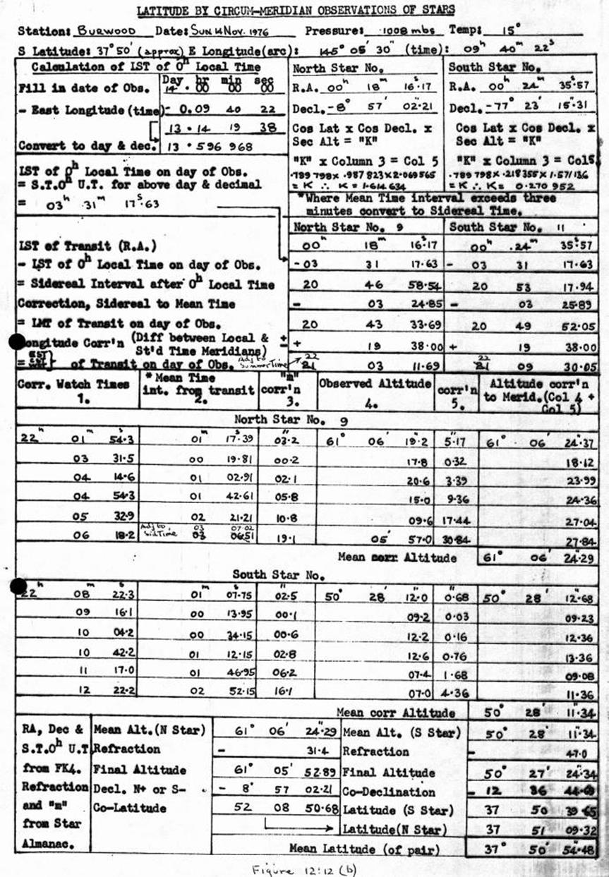
12.12 Latitude by Circum-Meridian Altitudes computation

A series of observations are taken on each star as explained in 3.13. Observations should commence no earlier and cease no later than 3 minutes from transit, with the attempt being made to have 3 observations on each side of transit. The observations are all on the same theodolite face and are balanced with similar observations on another star of equivalent altitude which bears 180° from the star initially observed. Figure 12.12(a) illustrates the method.

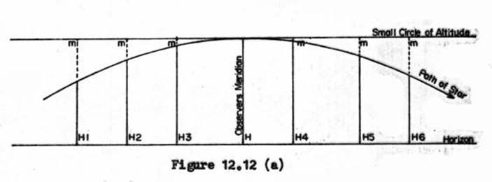
As shown above, when a star is close to transit, the small circle of altitude and the horizon can be considered parallel lines, as also can the altitudes H and HI to H6. Thus the requirement is to calculate the correction "m" for each observation so that when "m" is added to the observed altitude, the result is as though the actual observations were all taken at the time of transit. Knowing the accurate Longitude, from the FK4 it is easy to ascertain the time of transit of the star and using a stopwatch and time signal it is easy to ascertain the time of each observation. Using the small time difference between times of observation and transit, (i.e., Hour Angle) "m" can be found from a table in the Star Almanac, (or a more comprehensive table in "Close").

The formula for this table is :

Correction (seconds of arc) = 2*Sin²(½HA) / Sin 1" where ½HA is secs arc.

"m" is affected by the Latitude, also the Declination and Altitude of the star, therefore "m" from the table must be multiplied by a factor "k" obtained from :

Cos Lat x Cos Dec. x Sec. Alt.

The calculation is easy but must be methodically laid out as a separate "m" for each of the six observations must be read from the Table and then multiplied by "k" before applying the correction to each of the observations.

The attached proforma is ideal, as the worked example shows.
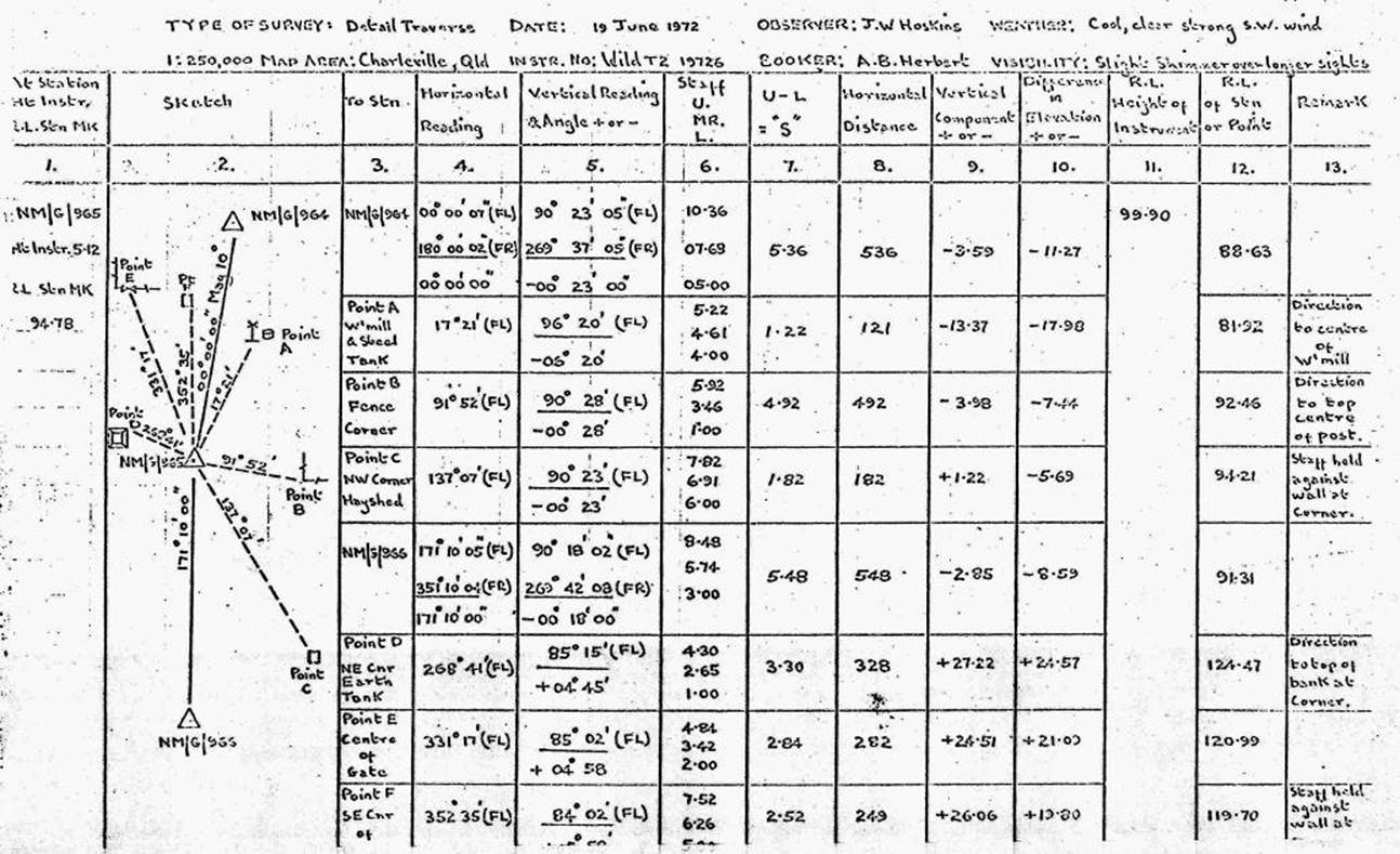
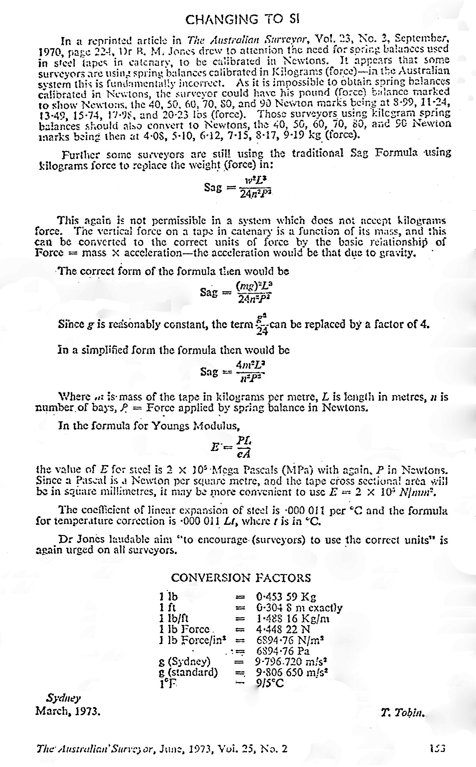