Airborne Electronic Distance Measuring :
A Brief History
Compiled by Paul Wise, 2016, revised 2022
Introduction
This paper seeks to catalogue the major airborne distance measuring systems that were developed during the twentieth century. After World War Two such systems were at the forefront of surveying technology until the advent of satellite-based surveying and navigation technology in the 1970s. This catalogue of airborne distance measuring systems is not exhaustive, with the focus on the history and use of airborne distance measuring systems used in, or associated with, the surveying and mapping of Australia.
Electro-optical distance meters were developed from techniques used to determine the velocity of light. The French physicist Armand Hippolyte Louis Fizeau (1819–1896) determined the velocity of light in 1849 with his famous cogwheel modulator on a line of 17.2 kilometres length. This experiment employed for the first time the principle of distance measurement with modulated light at high frequencies. Hans Zetsche (1979), stated that the first electro-optical distance meter was developed by Lebedew, Balakoff and Wafiadi at the Optical Institute of the USSR in 1936. In 1940, Alfred Huttel published a technique for determining the velocity of light using a Kerr-cell modulator in the transmitter and a phototube in the receiver. Huttel’s work inspired the Swedish physicist, Dr Erik Osten Bergstrand to design the first Geodimeter in 1943 to determine the velocity of light (Bergstrand, 1949 and Bjerhammar, 1972), the name Geodimeter was derived from Geodetic Distance Meter (Rueger, 1990).
Electronic Distance Measuring (EDM) is a term that evolved to describe any electro-optical device or system used to measure distance. Initial terrestrial and later airborne EDM and the speed of light have thus been inextricably interdependent. To determine a value for the speed of light the distance between two points had to be precisely known. Then, with the right equipment and the known value for the speed of light the distance between any two points could be determined. As radar based EDM equipment was perfected and calibrated against lines of already known length, the differences in length, known versus observed, indicated that the value for the speed of light needed to be revised. Because of that nexus, this paper contains a section on refinements of the value for the speed of light stemming from EDM development.
In compiling this paper, a considerable volume of material was reviewed. The material ranged from published books to personal accounts; and the facts were not always consistent or referenced. To provide the most accurate account, original documentation was sought and this forms the basis of the paper. Where matters of fact are described they are referenced allowing the provenance to be judged by the reader should other versions of the facts be read elsewhere.
The names of many of the systems discussed here are acronyms. Generally, such names should be spelt in capitals. However, RADAR has developed into common use and today radar is usually written in lowercase. In this paper, the common presentation of words is used and most system acronyms have only the first letter capitalised, for example Shoran. For clarity and consistency, the acronym CSIRO for Commonwealth Scientific and Industrial Research Organization is used. However, prior to 19 May 1949, this organisation was the Council for Scientific and Industrial Research (CSIR) and even earlier it was the Commonwealth Institute of Science and Industry and the Advisory Council of Science and Industry.
Electronic Distance Measuring
Obtaining distance from electronic instruments is fundamentally based on the measurement of the time taken for a signal to travel from an instrument at one station to a distant point and, after reflection or retransmission there by another instrument set at the point, to travel back to the transmitting instrument. Alternatively, the difference in phase between the transmission signal and the reflected signal as it leaves and returns to the instrument at the transmitting station, is measured. When the time taken and the velocity of travel of the signal are known, the distance between the two sets of instruments can be calculated. The signal is in the form of electromagnetic radiation and depending on the purpose the wavelength of the radiation chosen is generally categorised as being a radio wave, microwave, including radar, infrared or visible light, including laser. In its infancy, airborne EDM was known as radar ranging as radar wavelengths were used.
The velocity of travel of electromagnetic radiation is commonly known as the speed of light. Light is just a section of the Electromagnetic Spectrum that our eyes can sense and give us vision. Outside this section within the Electromagnetic Spectrum we have invisible microwaves and radio waves at one end, and at the other end of the Spectrum we have the invisible X and Gamma-rays. As light is visible, the speed of light can be measured and this value was quoted as the velocity of all electromagnetic radiation. However, as methods were refined, the value for the speed of light was regarded as the maximum value. But only in a vacuum (in vacuo) would all electromagnetic radiation travel at that speed. Generally, EDM signals have to transit the earth’s atmosphere and the friction caused by travelling through that medium reduced the transit velocity. The closest, practical calculation of this slower speed is given by formulae which use actual air temperature and pressure values to model the atmosphere at the time of measurement for the type of signal emitted. Thus, values for the speed of light vary depending on whether they are in vacuo, or are from actual free atmosphere measurement or are from measurements corrected, fully or partially, for atmospheric effects. To avoid confusion, the values for the speed of light quoted in this paper contain a reference to their source or can be considered as the in vacuo value at that time. Further detail on atmospheric corrections and their application can be found in Rueger (1990).
Initial World War Two Developments
In 1889, Heinrich Rudolf Hertz (1857-1894) a German physicist, concluded that solid objects interfered with, and scattered radio waves. Thereafter it was suggested from time to time, that this scattering might be used for locating obstacles. It was 1932 however, before British Post Office engineers observed the reflection of radio waves scattered from an aircraft in flight. Radar (RAdio Detection And Ranging) which can be described as the science of locating distant objects by radio, was proved by Great Britain during World War Two.
The breakthrough came with the invention of the magnetron in 1940. Until then the triode tube amplifier was used in many communication devices and was the basis of the first search radar systems. Because of transit time limitations, triodes were limited to radio frequencies. Greatly improved performance could be realised by operating at higher, microwave frequencies, however no suitable device was then available. The existing klystron, invented by the Varian brothers Russell and Sigurd in the United States, was not yet capable of sufficient power for radar applications.
John Turton Randall, Henry Albert Howard Harry Boot, and James Sayers at Birmingham University in England, extended the basic idea of the klystron. Their multi-resonator concept of the magnetron was an extension of the two resonator klystron. By late February 1940, they had constructed a new type of cavity magnetron, with a radiation wavelength of 9.8 centimetres. By May 1940, an experimental radar set using a pulsed, 10 centimetre wavelength, cavity magnetron had been built at the United Kingdom’s Telecommunications Research Establishment. The new radar was successfully tested by September 1940. This work resulted in the Plan Position Indicator (PPI), which even today we recognise as the most common type of radar display as shown in the diagram below.
The basic PPI has the radar antenna at the centre of the display, thus distances from the antenna are shown as concentric circles. As the radar antenna rotates, a radial trace on the PPI sweeps the dial in unison with the antenna and maps any reflections. Equivalent PPIs, called the Jagdschloss and Wassermann with a wavelength of 2 metres were developed by Germany. Such radar systems that just detect the radiation reflected from an object are called primary radar. In contrast, most of the EDM systems that are discussed below are classed as secondary radar. Secondary radar systems not only comprise a transmitter but, depending on the system, have one or more responders. These responders receive the transmitted signal and retransmit it, or respond to it. At the primary transmitter, the returned signals are received and interrogated to provide the distance information.

Generic diagram of a Plan Position Indicator (PPI) the basis of a search or primary radar.
The wartime technology push saw the PPI followed by the British Gee, OBOE, Decca and Gee-H systems, the American Loran, Raydist and Shoran as well as Germany’s and others own radar developments.
Gee
A blind landing system, using two synchronised transmitters, was proposed by Robert Bob James Dippy, in October 1937. At the time, Dippy was working at Robert Watson-Watt's radar laboratory at Royal Air Force, Bawdsey in the United Kingdom. The wartime requirement for navigation aids rather than landing aids led to a new proposal by Dippy on 24 June 1940. The original landing system design had used two transmitters to define a single line in space, down the runway centreline. In Dippy’s new concept, charts would be produced illustrating not only the line of zero difference, where the radar blips were superimposed like the landing system, but also a line where the pulses were received 1 microsecond apart, and another for 2 microseconds, etc. The result would be a series of lines arranged at right angles to the line between the two stations. A single pair of transmitters would allow the navigator to determine which line they were on, but not their location along it. For this purpose, a second set of lines from a separate transmitting station would be required. Ideally these lines would be at right angles to the first, producing a two dimensional grid that could be printed on navigation charts. To facilitate deployment, Dippy noted that the station in the centre (A) could be used as one side of both pairs (C and B) of transmitters if they were arranged like the letter L, as shown in the map below. Measuring the time delays of the two outlier slave stations relative to the centre master, and then looking up those numbers on a chart, an aircraft navigator could determine his aircraft’s position in space or get a position fix. The gridded lines on the charts gave the system its name, Gee for the letter G in Grid.
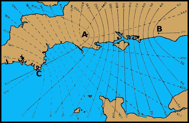
Map of southern England showing a superimposed Gee lattice with Master station at A and Stations at B and C as the outlier slaves (after Bowen, 1954).
To cover a wider area without having to run cabling hundreds of miles to connect all the transmitters, Dippy described a new system using individual transmitters at each of the stations. One of the stations, a master, would periodically send out its signal based on a timer. The other stations, slaves, would be equipped with receivers listening for the signal to arrive from the master station. When the slave stations received the master’s signal, they would respond by sending out their own broadcast. This would keep all the stations synchronised wirelessly. Dippy suggested building installations with a central master and having its three slaves about 80 miles (130 kilometres) away and arranged roughly 120 degrees apart, forming a large layout in the shape of the letter Y. A collection of such installations was known as a chain, an example of which is shown in the map below.
Experimental installations were already being set up in June 1940, and by July 1940 the system was usable to at least 300 miles (450 kilometres) at altitudes to 10 000 feet. On 18 August 1941, British Bomber Command ordered the Gee aircraft sets into production at Dynatron Radio Limited and Cossor Radar Limited, with the first mass produced sets expected to arrive in May 1942. In the meantime, a separate order for 300 handmade sets was placed for delivery on 1 January 1942 which was later pushed back to February 1942. Overall, 60 000 Gee sets were manufactured during World War Two. These sets were used by the Royal Air Force, the United States Air Force and the Royal Navy. A Gee Mark II was also developed to overcome jamming. By the time it became operational in February 1943, it had been selected for use by the United States 8th Air Force.
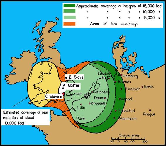
Map indicating coverage of a typical Gee chain in northern Europe (after Bowen, 1954).
By 1948, seven Gee chains existed: four in the United Kingdom, two in France and one in Germany. Gee developed into one of the most widely fitted airborne radio navigation aids of the day. Mobile transmitting stations for Gee were also developed. The first of these went into operation on 1 May 1944 at Foggia in Italy, and was used operationally for the first time on 24 May 1944. Other units were sent into France soon after D-Day. Preparations started for Gee transmitters in Nablus, Palestine, to guide flights across the Middle East but world events removed this requirement. Gee was finally shut down by 1970 but the principles behind Gee became the basis for what are generically called Hyperbolic Systems.
Bob Dippy's expertise saw him later recruited to the staff of the Woomera Rocket Range in Australia. During the instrumentation period Dippy joined the Long Range Weapons Establishment (LRWE) in late 1957 as Principal Officer in the Radio Frequency Techniques Group. Dippy was soon given overall authority for timing and his first task was to establish a dedicated timing section in his group, renamed Electronic Techniques (ETQ).
Hyperbolic Systems
These navigational systems required three ground stations with the necessary equipment as well as equipment in the mobile element be it vessel or aircraft. The measured quantity was the difference in distance between two fixed stations and the mobile element. This difference did not fix the position of the mobile element but defined a hyperbola, with the ground stations as foci, on which the position of the mobile element must lie. Consequently, the third ground station was required, and the observations of the difference in distance from it and from one of the other two stations to the mobile element then defined another hyperbola on which the mobile element must also be situated. Hence, the position of the mobile element was given by the point of intersection of the two hyperbolae. As with the Gee system, the hyperbolic systems’ ground stations were not independent of one another, and the use of master and slave ground stations meant that they were interlocked so that the choice of ground sites for this system was limited. This limitation was overcome, however, by establishing a chain of ground stations.
The Americans were not far behind the British Gee implementation with the development of their own system. Loran (Long Range Navigation), now identified as Loran A, was developed by the Radiation Laboratory of the United States Massachusetts Institute of Technology during 1941. This development work was supervised by the National Defense Research Council. Around mid 1942, Bob Dippy went to the United States for eight months to assist in Loran development. Many of the techniques Dippy used in Gee were adopted, and it was Dippy who insisted that the Loran and Gee receivers be made physically interchangeable so that any Royal Air Force or United States of America Air Force aircraft fitted for one could use the other by simply swapping units. This was to prove invaluable long after the war had ended, as Transport Command navigators flying the Australia run from the UK could plug in the appropriate set depending on where they were.
The first demonstration of Loran A was on 12 June 1942, with equipment installed on the airship K-2. This was followed on 4 July 1943, by the first readings from a Boeing B-24 aircraft. The first observations from a ship were made on a Coast Guard Cutter from 18 June to 17 July 1942. The observations during that period indicated a total range of 1 400 nautical miles was achievable with Loran A. These results were considered good enough to warrant the expansion of the system and its recommendation to navigational agencies. On 1 January 1943, the administration of Loran A was officially transferred to the United States Navy.
The range and relatively high order of accuracy of the Loran A system came from its use of the more stable and reliable propagation characteristics of radio waves. The Loran A system could be used for distances up to about 1 400 nautical miles at night and 700 nautical miles by day, with an accuracy of better than 0.25 nautical miles or 450 metres. Although useful for ordinary navigational purposes, Loran A was not accurate enough in itself for survey work. Consequently, the United Sates Coast and Geodetic Survey, Radiosonic Laboratory, later evolved an Electronic Position Finder (EPF). The EPF combined the main features of the shorter range Shoran with those of the longer range Loran system, so that it was now possible to fix the position of a survey ship accurately enough for hydrographic charting purposes. This system was initially called the Radio Ranger and after two years of testing and modification, it was used operationally in the Gulf of Mexico in 1947. The system was capable of 50 to 75 metre accuracy at ranges out to 300 kilometres.
In 1938 in Germany, Dr Ernst Kramar (said to have been working at Standard Elektrik Lorenz) developed an improved version of the Radio Ranger. However, as Standard Elektrik Lorenz (SEL) did not exist until 1958, Kramar was more likely to have been employed by its predecessor C Lorenz AG (AG was short for Aktiengesellschaft, the German equivalent of Corporation). Kramar's initial hyperbolic system was called Elektra and a later improved version was called Sonne (Sun). Operating at other frequencies, there was also to have been Mond (Moon) and Stern (Star). Sonne was installed in Norway, France and Spain as a navigational aid both for German aircraft flying the circuitous route over the Atlantic between France and Norway, and for the German U-boats. Following their acquisition of Sonne charts and a receiver, the British made use of Sonne under the name of Consol meaning by the sun. (See Proc (2015) for a summary of other hyperbolic radionavigation systems.)
Germany didn’t persist with hyperbolic radionavigation systems after World War Two. In contrast, the United States Loran A network consisted of over 70 transmitters and provided coverage over about one third of the earth’s surface. In the late 1940s and early 1950s, experiments in low frequency Loran produced a longer range, more accurate system. Technical problems resulted in Loran B never becoming a commercial system and was eventually surpassed by Loran C. Loran C provided longer range and greater accuracy when it first came into operation in 1957. Using the 90-110 kHz band, Loran C operated in parallel with Loran A until the mid 1970s, providing navigation assistance throughout the area shown on the world map below. The United States continued operating Loran C until the network’s closure in the mid 1990s.
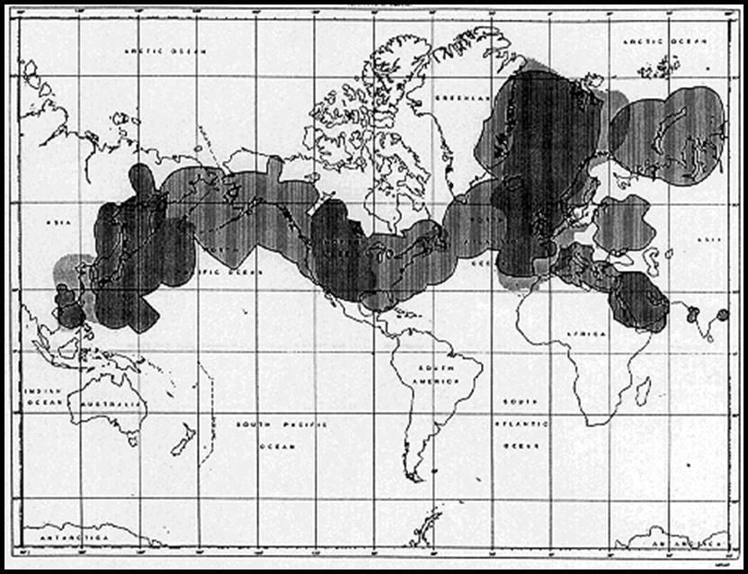
Map illustrating the global coverage of Loran.
(from Proc (2015) originally attributed to Eurofix web page).
From 1936 to 1939, William Bill Joseph O'Brien had been working independently on a method of measuring the ground speed of aircraft. His system was called the Aircraft Position Indicator (API). At the outbreak of World War Two the American government and civilian authorities were uninterested in O'Brien’s API. O'Brien then offered his idea to the British Air Ministry through his friend Harvey Fisher Schwarz. Schwarz was an American then working in London for the Decca Record Company Limited. This company was previously known as the Decca Gramophone Company Limited and had a sister company Decca Radio and Television Limited, both of which were London based. The later success of O’Brien’s work spawned the Decca Navigator Company. With this proliferation of the Decca name, and with some equipment bearing only the brand name Decca, it is often difficult to trace the exact source of some Decca equipment.
With D-Day looming, the British Admiralty wanted to guard against the jamming of their Gee system and so took an interest in O'Brien’s API in 1941. Trials were organized off Anglesey in mid 1942 using a master unit transmitting at 300 kHz and a slave unit transmitting at 600 kHz. Successful comparison of the signals was made at 1200 kHz and further research by Decca Radio and Television Limited was then undertaken with assistance from the Admiralty Signals Establishment. Early in March 1943, Decca was given the order to produce 27 receivers plus the driver and phase control units needed for the transmitters. All equipment was delivered by mid May 1943 when the Royal Navy began its D-Day training and preparations in earnest. In January 1944 a test of Decca on new frequencies was carried out in the Irish Sea and it was also compared with the Royal Air Force Gee system for accuracy. Although Gee and Decca were similar in broad principles, Decca was considered more accurate than Gee and in today’s terms more user-friendly, because the results were presented directly on clock dials called decometers instead of a cathode ray tube as in Gee. A photograph of Decca’s decometers is shown below. One disadvantage of the early Decca sets was the need for the decometers to be initially set up using an accurately known position. If there was a break in reception for any reason, the decometers had to be recalibrated.
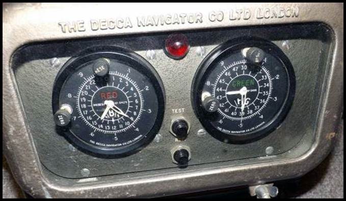
Decca’s decometers.
Post war, the Decca system was largely applied to hydrographical surveying. Ranges up to 400 miles (650 kilometres) were obtained over water. The accuracy varied with the position of the point to be fixed relative to the three shore stations. Experience showed it to be suitable for both inshore and offshore hydrographical work. Decca was also used satisfactorily for tracking strips of aerial photography for British Ordnance Survey’s large scale mapping. Decca’s range and accuracy came from it operating on wavelengths of several kilometres. These low frequency wavelengths tend to follow the earth’s curvature for very long distances at a speed of propagation mainly related to the medium over which they travelled. Decca was adapted for best accuracy over sea water. However, over land with its constantly changing density and nature of the earth's surface, the same accuracy could not be replicated.
Raydist, from a mix of the words Radio and Distance was a post war system, first mentioned as being in development on 18 April, 1947. The system was developed by the Hastings Instrument Company of Hampton, Virginia USA, which was founded in 1944. The hyperbolic type N (for Navigational) Raydist permitted multiple users in the same net and gave an accuracy of about 15 to 30 metres at a distance offshore of 80 kilometres. A type DM (for Distance Measuring) Raydist was produced as well as other variants. The DM Raydist operated at 3 MHz and was accurate to under 1 metre at over 400 kilometres. In the days before GPS, DM Raydist was used to calibrate the Inertial Navigation Systems on early nuclear submarines.
OBOE
While Gee had successfully impacted wartime aircraft navigation, cloud below 20 000 feet obscuring the target meant a stand down which frustrated the commanders and aircrew of Bomber Command. British wartime Prime Minister Churchill thus gave high priority to developing improved methods of navigation and accurate payload delivery despite cloud or haze. OBOE was proposed by Alec Harley Reeves and his co-worker Frank Jones at Britain’s Telecommunications Research Establishment. Operational in late 1942, the OBOE system required two transmitters initially based at Dover and Cromer. The two ground stations both emitted streams of pulses on the same carrier frequency, but at differing intervals. The aircraft carried a responder, which replied to the interrogations of both ground stations so that each ground station knew the range to the aircraft. Operationally, the aircraft flew a course of constant radius about the tracking station Dover, the course radius being such as to bring the aircraft over the target. When the aircraft arrived at a precise distance from the releasing station Cromer, a signal was sent automatically which released the payload. Please refer to the diagram showing OBOE’s operating principle, below. The pulses from the tracking station were commonly sent at a frequency of 133 pulses/second and modulated by Morse signals to convey information to the aircraft’s crew. Thus if the aircraft was at too short a range a series of dots was sent. If at too great a range, a series of dashes was sent. When the aircraft was on track a constant tone like that from the orchestral instrument the Oboe was heard. Hence the name OBOE. The technology, however, limited the use of OBOE to one aircraft at a time. Germany improvised a system conceptually similar to OBOE, code named Egon.
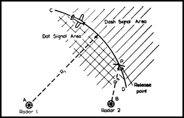
OBOE’s operating principle (after Bowen, 1954).
It is interesting to note that even in these early days of airborne EDM that the historical, insular, territorial map datums caused problems. Such were the differences between these datums that they could be detected indirectly by these early airborne systems (Bowen, 1987). Based on existing map data, point to point distances across historical map boundaries would be determined. The radar would then direct an aircraft based on those distances. European map datums caused the determined distances to be incorrect and as a consequence the required location was not being overflown. Once a datum difference had been identified and quantified, appropriate operational adjustments could be made. Although unknown at the time, this was probably the first attempt at comparing intercontinental map datums. Please refer Annexure A.
Gee-H
The name Gee-H is confusing, since operationally the system was similar to OBOE and not very much like Gee. The name was adopted because the system was based on Gee technology. It operated on the same range of 15 to 3.5 metre wavelengths or frequencies of 20 to 85 MHz, and initially used the Gee display and calibrator. The H suffix came from the system using the twin-range or H-principle of measuring the range from responders at two ground stations. While Gee-H was about as accurate as OBOE with a range of about 300 miles it could be used by as many as 90 aircraft at once. For this number of aircraft to uniquely recognise the responses to their own transmissions, the pulse recurrence frequency was jittered automatically, that is the inter-pulse timing was altered. Only the signals with the same interpulse timing would be recognised by the device in a particular aircraft. The time taken by a ground station to receive a pulse, send out the response and return to the receiving condition, was about 100 microseconds. With a pulse recurrence frequency of 100 cycles/second a ground station would be busy for 10 000 microseconds in any one second dealing with the enquiries of one aircraft. A Gee-H ground station would therefore have 990 000 microseconds free in each second in which to respond to other aircraft, giving a theoretical maximum handling capacity of 100 aircraft. When Gee-H became operational in 1944, maximum handling capacity of the stations was not achieved hence the more practical limit of around 90 aircraft per station was adopted.
The Gee-H system required two ground stations already fixed by ground survey methods and about 100 to 120 miles (200 kilometres) apart. The aircraft carried a pulse transmitter and receiver and pulses were sent to each ground station responder in turn. The responders returned the pulses to the aircraft on a different frequency. Here the return pulses were received and the time interval between transmission and reception was recorded or measured. The transmission of pulses, that is intense bursts of energy which lasted a very short time and were then repeated after a relatively long period, gave the radiated energy time to travel to the distant responder and then return to the transmitter’s receiver before the next burst was emitted. In this way, no confusion or interference in reception was likely to arise between the outward and returning signals. With a suitable electronic display and a large number of repetitions of the bursts, the emitted and received signals could be made to form images which could be seen by eye or could be photographed as a continuous picture. The derived measurements gave the distance from the aircraft to each ground station responder. With the height of the ground stations known from the ground survey data, and that of the aircraft obtained from altimeter readings, the aircraft to ground distances could be easily reduced to the equivalent arc lengths at sea level. Accordingly, the lengths of the sides of a spherical triangle became known and the triangle could, if necessary, have been solved to give the three respective internal angles.
Transmitters on the ground as used by OBOE, meant that the ground equipment could be larger, more complex and powerful. Smaller, lighter transponders went into the aircraft. The signal information was thus distributed between two ground stations, while other important information like altimeter readings, was collected in the aircraft. Recording therefore had to be done at three points and the times correlated. It was found more preferable to retain the transmitter in the aircraft and focus all the data gathering there as with Gee-H.
The wartime need to make maximum use of existing Gee equipment in Gee-H, while practical, forced the use of less accurate, lower frequencies. To obtain greater accuracy a higher frequency should have been chosen. When designed, the American Shoran system was able to employ a higher frequency and replace Gee-H.
British Colonial Mapping with Gee-H
As in wartime, the ability of Gee-H and the later Shoran system to fix the position of an aircraft was found to be just as advantageous in peacetime. The mapping of dangerous or hard to reach places, or where traditional survey and mapping was just not possible, could now be achieved using airborne methods. By judiciously establishing a relatively few fixed points on the ground to site responder beacons, vast regions could be accurately photographed from the air almost without needing to set a foot on the ground.
Initial development work was carried out by the War Office from 1943-45 when British Brigadier Martin Hotine was Director of Military Survey. Investigations were carried out in cooperation with the British Air Ministry, the Ministry of Aircraft Production, and the Telecommunications Research Establishment. These investigations were supported by Survey Units of the Royal Engineers, Royal Canadian Engineers and the United States Corps of Engineers and others. British Major Cecil Augustus Hart was responsible for the research work related to surveying.
With the transmitter and measuring equipment in the aircraft the capability of Gee-H made it ideal for use in the British Colonies. Under the Directorate of Colonial Surveys, photogrammetric mapping on the scales of 1: 50 000 and 1: 25 000 was successfully undertaken in Ghana, Gambia, Sierra Leone, Rhodesia, Nigeria, Gold Coast and Tanganyika. Topographic maps were needed for various colonial development schemes. These schemes included a railway link between East and Central Africa, irrigation projects in Basutoland, hydroelectric undertakings in Rhodesia and West Africa, international boundary definition, and agricultural and mineral developments in other parts of the African continent.
From 1946 to 1952, No.82 Squadron of the Royal Air Force had its base near Nairobi in Kenya. The Squadron was equipped with seven Avro Lancaster MK.1 aircraft for photography operations. Its two Douglas Dakotas handled passenger and freight carrying tasks. The Dakotas were also used for supply-drops to the parties manning the remote Gee responder beacon sites. The Squadron initially used the American K17 aerial survey camera but in August 1951 changed to the F49 being the RAF designation for the Williamson Eagle IX aerial survey camera. The improvement in photographic quality was most noticeable due to the Williamson camera’s improved optics and the pressure-plate system for holding the film in perfect register with the focal plane. With a six inch focal length lens, a nominal photoscale of 1: 30 000 could be achieved except in extreme cases as the Lancaster’s were incapable of reaching altitudes above 23 000 feet.
It had been initially hoped that, by using two radar stations, it would be possible to fix the positions of the photographs with sufficient accuracy to allow the maps to be plotted without surveyors going in on the ground. Although this was done later in Gambia, it was generally found to be impractical (Macdonald, 1996).
Four mobile Gee-H responder units gave the aerial photographic program flexibility of operation. The Gee-H responder sites were situated on suitable high points whose position was fixed by prior astronomical observation. Operationally, the aircraft was guided by the navigator with his Gee-H unit towards an established ground responder. At the predetermined distance from the responder the aircraft would be turned onto a course for the photography acquisition. This course would be the arc of a circle so the aircraft was continuously turning. The Gee-H unit would indicate any deviation from the set course. A near vertical photograph was required about every 20 seconds. Accordingly, just before an exposure a red light showed in the cockpit to warn the pilot to fly the aircraft exactly level for that instant, before returning to course. For the aircrew it was a difficult and exhausting task. Owing to this mode of operation over circular tracks, it was impossible to work closer than 30 miles to the Gee-H responder. Conversely, owing to erratic reception, operations were unsatisfactory at distances much greater than 200 miles from the Gee-H responder. Accurately plotted ground control points in addition to the Gee-H responder beacons were used to relate the acquired photography to the ground to confirm coverage or indicate gaps. Please refer to the photograph below. Even the most expert aircrews failed to get perfect coverage and filling in the gaps was the most difficult job of all. More detail including specifications and operational requirements can be found in Hellings’ 1954 paper Radar Controlled Air Survey Photographic Operations in Africa 1946–1952.
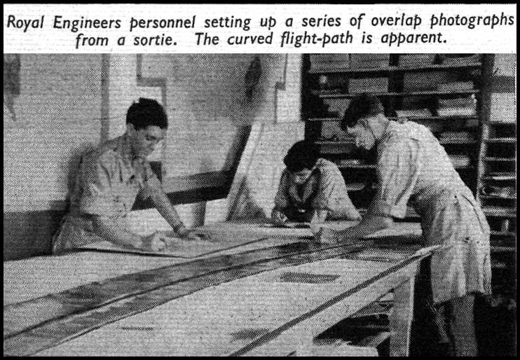
Courtesy Flight Magazine, 14 November 1952.
The total area covered during the whole six years of operation was 1 216 000 square miles. This involved an average of 8 000 negatives taken and processed each month and the operating of Gee-H responder beacons at 44 separate locations. In addition to the large aerial photographic program in Africa, a Mosquito Squadron, based on Singapore, flew similar photographic operations in Malaya, North Borneo and Sarawak.
Shoran
Across the Atlantic, the Americans had continued with their own wartime airborne EDM development efforts. In 1938, Stuart William Seeley an engineer with the Radio Corporation of America (RCA), found he could measure distances by time differences in radio reception. In mid 1940, Seeley proposed building Shoran for the US Army Air Force and by late 1944 Shoran was in operation in Italy.
The official long name for Shoran is SHort-RAnge Navigation, (Rabchevsky, 1984). However, former US navigators and bombardiers used the long form name SHort-RAnge Aid to Navigation.
During the system's development, Seeley and an RCA manager flew to England to describe the system to American and British Air Force personnel. There they observed the OBOE system which could only guide a single aircraft, whereas multiple aircraft could be guided by Shoran. The Shoran system, used carrier frequencies of 230 to 250 MHz (wavelengths of around 1 metre). By contrast, the British Gee and Gee-H systems worked on frequencies of about 30 to 43 MHz (wavelengths of 10 to 7 metres). With Shoran, the transmitting frequencies were switched in turn so that the ground station responders were alternately interrogated at intervals of a twentieth of a second, and both ground stations responded on a frequency of 300 MHz. The intervals were regulated by crystals in the responders which were thermostatically controlled, and by a crystal in the aircraft which was calibrated against the responders while in operation. A positional accuracy of 20 yards in 200 miles (7 metres in 100 kilometres) or better than 1: 15 000 could be achieved. Kroemmelbein’s 1948 paper Shoran for Surveying, provides details of the Shoran electronics.
About the time Shoran became operational in 1944, a conference on the future uses of Shoran was held at Wright Field in Dayton, USA. Two of the attendees were Lieutenant Commander Clarence Burmister, US Coast and Geodetic Survey (C&GS), and Lieutenant Colonel Carl Aslakson, US Army Air Force. Aslakson was a C&GS officer who was transferred to the 311th Photo Wing for the duration of the Second World War. During 1944-1945, Burmister was active in converting Shoran to a hydrographic surveying system, while Aslakson pioneered the use of electronic systems for geodetic distance measurement beginning with Shoran.
Up to 1944, measuring ground to air distances was limited by equipment range and aircraft flying height. In 1945, Aslakson formulated the use of an aircraft to cross an imaginary line between two Shoran responders, hence the name line crossing technique. This technique had the advantage that much longer lines could be measured but the cost was the need for retransmitting equipment at each end of the line. The technique required an aircraft to fly across an imaginary line between two ground station responders, usually at a slight angle to it and near the centre. A series of simultaneous observations were taken at close intervals of time to each ground responder. With distances to the aircraft measured for a number of positions on each side of the direct line between the two ground stations, the sum of the distances was obtained. The results were plotted as a curve against time and the minimum sum for all possible positions of the aircraft on the line of flight obtained. More frequently however, the minimum sum was obtained analytically from a least squares solution. The minimum distance obtained after reduction to the arc length at sea level was the required length of the direct line. This method of measuring the lengths of long lines was known as radar ranging.
During all line crossing measurements, the aircraft was kept at a constant altitude as measured by an altimeter. The elevations of the end stations had to be known or determined by ground parties. Observations for pressure and temperature were taken at timed intervals at the ground stations and were also recorded in the aircraft.
The same method could be used for calibrating the airborne EDM equipment. Here the flights were made across a line whose length had already been determined by ground survey methods. The difference between the line length obtained by radar ranging and that determined by ground methods gave a correction which could be applied to other measurements made with the same equipment.
Using what Aslakson and Rice reported in their 1946 paper, Use of Shoran in Geodetic Control, as refined Shoran operating methods, six lines of a first order geodetic triangulation network were measured using the line crossing technique. With the elimination of any systematic error and by observing the line crossing for any given line more than five times at least, the precision of the determination of the length of a single line could be increased and an accuracy of something like 1: 20 000 (5 metres in 100 kilometres) obtained.
Between 1947 and 1949 Canada undertook the development of Shoran for surveying and mapping. The Royal Canadian Air Force (RCAF), National Research Council (NRC), Dominion Meteorological Service and the Department of Mines and Technical Surveys all participated in this development. Testing was conducted in the Ottawa area over several long lines of the Canadian first order triangulation network. The RCAF’s 408 Squadron was later tasked with the Shoran survey of Canada. The 408 (Goose) Squadron was a famous wartime unit. It was re-formed at Rockcliffe on 10 January 1949. The Squadron operated eight Lancaster MK.X modified aircraft, four of which were equipped with Shoran sets. The Shoran survey started with the measuring of the line between the points, Sprague and Camp Hughes, just South of Winnipeg, which were already tied into the United States own survey. These connections enabled the Shoran survey to use the North American Datum 1927 (NAD 27) with its origin at station Meades Ranch. Shoran then formed a trilateration connection with the survey at Edmonton. The resulting small survey misclose further validated Shoran’s capability. (Trilateration is a survey method where the lengths of the sides of triangles are measured. It is a different approach to the classical survey triangulation method where the angles within the triangles were measured.)
The Canadian Shoran survey took until 1957 to complete and provided the control required for 1: 250 000 scale topographic mapping in the remotest areas of Canada. Some 143 points were connected by 502 lines. The longest line was 367 miles. An overall accuracy of 1: 56 000 was achieved. Between the Shoran fixed points other minor control points were fixed from aerial photography by aerotriangulation, the latter points being adjusted to the points established by Shoran. Such was the success of this survey that when Shoran is mentioned the Canadian survey immediately comes to mind. A map showing the extent of the Canadian Shoran survey is at Annexure B, Map B1.
The Shoran airborne equipment as shown in the photograph below, weighed about 340 kilograms. With the addition of two operators the aircraft used had to carry a payload of some 600 kilograms. At each ground station there was a responder beacon, which with its power supply weighed 680 kilograms. Each ground station also required two operators plus a 250 litre drum of petrol to fuel the power generator.
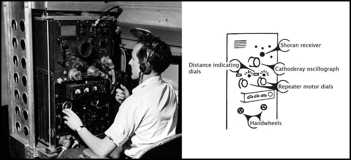
1949 photograph of operator with CSIRO with a Radio Corporation of America (RCA) Shoran aircraft receiver, ID-17/APN-3, in Douglas Dakota C47B aircraft, with explanatory diagram.
The following procedure was generally followed to achieve a Shoran line crossing. The aircraft navigator, who was provided with special equipment to enable him to know his approximate position at any moment, warned the Shoran operator when some distance away from the point where he expected the aircraft to cross the line. The Shoran operator then searched his oscilloscope to pick up the signals from the port and starboard responders at the ends of the line. These were called the drift and rate ends respectively. After picking up these signals, which were indicated by pips on a circular trace on a cathode ray tube, he followed them as the aircraft approached the mid point of the line. By turning two handles, the operator could bring the ground signals into coincidence with a marker pip and then kept all three in coincidence until the navigator informed him that the line crossing was complete. Meanwhile, shortly before he considered the aircraft was about to cross the line, the navigator switched on the recording camera. This camera photographed the dial panel of the Shoran set at prearranged intervals of three seconds, and after 60 frames were acquired, he switched the camera off again. This completed one line crossing. The photographs taken on 35 mm film, were subsequently enlarged to extract the recorded data. The frames showed the two dials where the distances to a thousandth part of a mile, or about 1 metre, to the drift and rate stations at the moment of exposure were indicated. Other dials included in the 35 mm photoframes recorded orientation, temperature, time and altimeter, the frame number and the run number. After four line crossings a second Shoran operator took over the duties of the first, and another four line crossings were made. On a separate day, and in theoretically different meteorological conditions, another sequence of two sets of four line crossings were made. Each line was therefore measured at least sixteen times in different atmospheric conditions.
The Canadian work showed that the ground station responder crystals needed to be calibrated before and after each working season, but were generally found to have kept their frequency to within 2 parts per million. A constant delay also occurred at each responder which was determined before and after each operating season. Even so, the resolution of Shoran meant that a single measurement could only be accurate to about 8 metres. Larger errors occurred with the variation of signal strength.
Around the end of World War Two, the then United States Army Air Force became interested in testing Shoran to determine whether it could be used for establishing survey control to geodetic standards. From this work emerged Hiran. Aslakson collaborated with Seeley of RCA, to design a modified Shoran system that would prove to have accuracies of better than 1: 100 000 (1 metre in 100 kilometres). For proof of concept, Aslakson set responders on known first order geodetic points and compared the Shoran derived distance to the known geodetic distance. He discovered a systematic difference that ultimately could only be explained by revising what was then the accepted value for the velocity of light (Seeley, 1961). This aspect is discussed in detail in the next section.
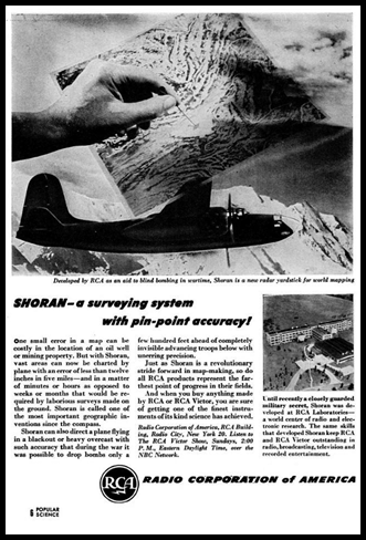
1946 Radio Corporation of America (RCA) advertisement for using Shoran for surveying.
Industry also saw Shoran as a valuable tool in the post war search for, and exploitation of, natural resources. Please refer to the advertisement above or version here. Surplus Shoran systems became widely used for navigation in the oil and gas exploration industry. Shoran equipment was deployed to navigate seismic survey vessels and position drilling rigs around the world. Truck-portable Shoran transponders with an antenna up to 90 feet tall (27 metres) were set up within a few feet of geodetic survey stations near the coast. Shoran chains consisting of three or four shore stations were used to provide highly accurate navigation across large exploration tracts that were up to 200 miles (320 kilometres) offshore. Frequently, the old massive vacuum tube transmitters were fitted with solid state control boxes for more reliable operation and to improve reception of weaker signals over the horizon.
Value for the speed of light
As mentioned earlier, a value for the speed of light was required to convert the time of travel for a Gee-H, Shoran or later Hiran/Shiran electronic signal to a distance. Table 1 below lists the values for the speed of light relevant to this paper. The list also shows the source of the listed value as the value can vary between references. Erik Bergstrand in his 1957 paper Some Recent Determinations of the Velocity of Light, also developed a best value for the speed of light which was very close to the final value adopted by the International Union of Geodesy and Geophysics and subsequently adopted by the National Mapping Council of Australia in March 1958.
|
Person & method |
Year(s) |
Speed of light in vacuo (kilometres/second) |
|
Albert A Michelson – optical |
1926 |
299 796 ± 4 (1) |
|
CA Hart (1948) after AA Michelson |
1929-33 |
299 774 ± 11 (1) |
|
Wilmer Anderson - optical |
1939-41 |
299 776 ± 4 (1) |
|
JJ Warner (1947) after RT Birge (*) |
1941 |
299 776 ± 4 (1) |
|
FE Jones & EC Cornford – OBOE |
1949 |
299 783 ± 25 (2) |
|
Erik Bergstrand - Geodimeter |
1949 |
299 796 ± 2 (4) |
|
Carl Aslakson – Shoran |
1949 |
299 792.4 ± 2.4 (3) |
|
Louis Essen - cavity resonator |
1950 |
299 792.5 ± 1 (2) |
|
Carl Aslakson – Hiran |
1951 |
299 794.2 ± 1.4 (3) |
|
Keith Froome - radio interferometer |
1951 |
299 792.6 ± 0.7 (4) |
|
Trevor Wadley – Tellurometer |
1956 |
299 792.9 ± 2 (4) |
|
Accepted |
Today |
299 792.458 (4) |
|
|
||
|
The values are taken from original papers (1) Warner 1947, (2) Essen 1952, (3) Aslakson 1951, and (4) http://www.ldolphin.org/cdata.txt. Also refer Bjerhammar (1972). |
||
|
Note (*) : JJ Warner was involved with Australian Shoran tests 1948-49. |
||
Table 1 : Measurements of the speed of light relating to airborne EDM.
As mentioned above, Cecil Augustus Hart had been responsible for the research work in developing airborne EDM for surveying. In his 1948 paper, Hart stated that the fundamental velocity of the propagation of light in vacuo had been derived by optical methods over many years. Hart added that a recent value accepted for radar navigation throughout the War was 299 774 ± 11 kilometres/second. Michelson and others (1935) derived this value from 2885.5 determinations of the velocity, during the period September 1929 to March 1933. These determinations were achieved despite Michelson’s death on 9 May 1931 when only 36 of the 54 series of observations taken during 1931, had been completed. Earlier, a 1924-26 series of measurements of the velocity of light had given a value of 299 796 kilometres/second which was interesting in the light of future events; please refer to Table 1 above.
During 1946, the British had carried out experiments using OBOE from a station in North Devon and a Mosquito aircraft. Firstly, the Mosquito was flown across an extended base line between two geodetic stations as nearly as possible on a predetermined tracking range. Then the aircraft flew tracks of three different radii from the OBOE station. There had also been earlier experiments using Gee-H during the war over two ranges in the South of England. Gee-H equipment, although less accurate than OBOE had to be used for operational reasons. The main purpose for these tests was to gain data on how flying height and distance from the responder beacon affected the speed of light.
When the values for the speed of light that resulted from all of this work were used to compute distance they gave measures of accuracy for OBOE and Gee-H within the range of 5 to 13 metres. Francis Edgar Jones and EC Cornford (Hart, 1948), are credited with concluding that their airborne EDM distances only matched already surveyed distances if the value for the velocity of light was increased by nearly 14 kilometres/second. That is from Michelson’s accepted value of 299 774 kilometres/second up to 299 788 kilometres/second.
Following the development of Shoran in mid 1945, a British-American team used Shoran to measure a 618.369 kilometre line in Italy. The American Shoran system used Wilmer Anderson’s 1939-41 value of 299 776 kilometres/second for the speed of light in preference to the earlier British value of 299 774 kilometres/second used in OBOE and Gee-H. In this experiment the aircraft was flown 22 times across the line between the ground station responders. During each crossing the minimum distance was observed, and later reduced to a sea level distance. The line crossings were made at altitudes of 11 000 and 15 000 feet. The mean of the Shoran derived distances was 618.320 ± 3.5 metres an accuracy of only 1: 13 000. If Essen's later value of 299 793 kilometres/second for the speed of light were used instead of the 299 776 for which the Shoran computer was designed, the discrepancy would have been reduced to 5 meters, an accuracy of better than 1: 120 000.
In mid 1949, Aslakson reported on his most recent Shoran work. A network of 47 lines varying in length from 67 miles to 367 miles (105 kilometres to 590 kilometres) were measured using the line crossing method. Six of the lines measured could be directly compared with geodetic distances previously obtained from first order triangulation. The entire network however, was so designed that a rigid adjustment was also able to be made. From the comparison with the six geodetic lengths and from an adjustment of the 41 other lines, a value for the speed of light of 299 792.4 kilometres/second was derived. Using this new value for the speed of light the accuracy on 41 of the 47 lines exceeded 1: 25 000 (4 metres in 100 kilometres).
To achieve the above results, refined Shoran measuring and distance derivation procedures had been adopted. Specifically, flying the line crossings so as to eliminate observer's errors, using a least squares computation to calculate the minimum sum distance, improving the measuring of the aircraft’s altitude, applying an atmospheric correction based on actual airborne weather reconnaissance at the time of the line crossing, and modifying the geometric corrections for the reduction of the slant Shoran distances to sea level distances or to the approximate geodesic. These procedures were in addition to extensive instrument research that resulted in numerous modifications of the Shoran system. The most important of these was the discovery of an error which was due to changes in the intensity of the signal and the design of a method to correct for this error. Many of the instrumental changes were suggested by RCA’s Shoran inventor Stuart Seeley. While some attempt was made to maintain signal intensity during this project it was not done consistently.
Nevertheless, the above improvements led to the development of what was to be later called Hiran. Hiran is discussed in detail in the next section. The first Hiran system was tested during February and March 1950, over a network of 15 lines in Florida. The accuracy of the Hiran measured lines was better than 1: 100 000 or 1 metre in 100 kilometres. From this work Aslakson also derived a new value for the speed of light being 299 794.2 ± 1.4 kilometres/second.
John James Warner of the Division of Radiophysics of CSIRO, authored a 1947 paper, The Velocity of Electromagnetic Waves. Warner examined the work of Raymond Thayer Birge in correcting various values previously found for the speed of light and establishing them on a common basis. Warner concluded that Birge’s value (refer Table 1 above) was probably the best at that time. Soon thereafter, Warner was to lead Australian tests of Shoran which are fully described below. Hart (1948) reported the results of early work over a single line, stating in Australia, experimental work has been carried out on a ground surveyed distance of first order accuracy of 158.812 ± 0.001 miles (some 256 kilometres). The mean of 46 radar line crossing measurements, when reduced geodetically, gave 158.848 ± 0.009 miles. At the time of writing the volume of experimental work is not sufficient to explain the discrepancy of 0.036 miles (nearly 58 metres or 23 metres per 100 kilometres). As will be seen later in this paper, by the end of the eighteen months of Australian Shoran testing the discrepancy had been reduced to around 7 metres per 100 kilometres.
As a result of all this work to determine an operational value for the speed of light to use with EDM, the then current value was still some 16 kilometres/second too slow! Aslakson (1951) adopted the value of 299 793 kilometres per second for future use with Shoran/Hiran. The report on the 1962-64 Southwest Pacific Survey, using Hiran, specifically recorded that a value of 299 792.5 kilometres/second was used for the speed of light.
|
Technology |
Year |
Quoted/Derived Accuracy(*) |
Location |
|
|
±m |
Ratio |
|||
|
Shoran |
||||
|
|
Wartime |
[20] |
1:15 000 |
Given as 20 yards in 200 miles |
|
|
|
|
|
|
|
1943 |
15 |
[1:20 000] |
Canadian trials, over lines 160-497 km |
|
|
1945 |
45 |
1:13 000 |
Italy, over 618 km, using 299,776 km/s for speed of light |
|
|
5 |
1:120 000 |
Italy, results improved if value for speed of light changed to 299,793 km/s |
||
|
|
1946 |
[17] |
1:17 500 |
Aslakson tests with wartime system |
|
|
|
[15] |
1:20 000 |
Aslakson tests removing systematic error |
|
1949 |
[4] |
1:77 000 |
Best accuracy from Australian tests over 350 km and some 10 crossings |
|
|
|
|
7 |
1:14 000 |
Accuracy of 7 parts per 100 000, concluded from Australian tests of modified Shoran. |
|
|
1949 |
[12] |
1:25 000 |
Aslakson testing improved Shoran, over lines 105-590 km on 47 lines network |
|
|
1957 |
[9] |
1:56 000 |
Canada - accuracy achieved by survey |
|
|
|
|
|
|
|
Hiran |
1950 |
[3] |
[1:100 000] |
Aslakson test of first Hiran, over lines 65-515 km on Florida network of 15 lines |
|
|
|
|
|
|
|
1950-53 |
[3] |
1:113 000 |
Florida ‑ Trinidad - Barbados link, line length not stated |
|
|
4 |
[1:75 000] |
Puerto Rico - Trinidad link, over lines 500-758 km |
||
|
|
|
|
|
|
|
|
1953 |
5 |
[1:60 000] |
Crete - Africa link, over lines 134-355 km |
|
1953-56 |
4 |
[1:75 000] |
America - Europe link, over lines averaging 440 km |
|
|
|
late 1950s |
3 |
1:160 000 |
Accuracy after final network adjustment as quoted in Lexicon on Geodesy and Mapping in AFHRA documents |
|
|
|
|
|
|
|
1965 |
4 |
1:131 000 |
AF 60-13, Southwest Pacific Survey, 1962-64, using 299,792.5 km/s for speed of light |
|
|
|
|
|
|
|
|
Shiran |
early 1970s |
1 |
[1:300 000] |
Not stated but probably Brazil |
|
(*) Values in square [] brackets have been derived from the quoted value using a standard distance of 300 kilometres |
||||
Table 2 : Comparison of Shoran, Hiran and Shiran accuracies.
Hiran
Hiran (officially HIgh-precision ShoRAN, Rabchevsky 1984), but again sometimes unofficially HIgh frequency RAnging and Navigation), was the technological evolution of Shoran but the evolution also generated the more user-friendly Shoran sets of the late 1950s. These advances primarily reduced the workload of the airborne Shoran operator. Aslakson (1951) stated that in February and March 1950, the United States Air Force completed an extensive project in Florida, wherein modified Shoran equipment was tested. Aslakson (1980) further stated that following the last tests of the Hiran equipment and the issuance of the final report of the 7th Geodetic Control Squadron at Orlando, Florida, they considered themselves competent to undertake an important geodetic connection across the Atlantic to Canada via the Greenland Ice Cap. Much to Aslakson’s disgust, this project of 1950 was a complete failure due to inexperience resulting in insufficient azimuth control being acquired. The resurvey was completed in 1956.
It will become clear that Hiran was only used by the United States Air Force. Thus any other project said to have used Hiran had in reality used advanced Shoran, that is the more user friendly Shoran but without the addition of the resource overhead of the complex ground and air gain control instrumentation. Likewise, in the early 1950s some surveys are shown as using Shoran when it is highly likely that they were using Hiran before that name was adopted, or even a mix of Shoran with later Hiran to improve the final accuracy. Table 2 above was thus compiled on the basis of Hiran being used from 1950 by the United States Air Force, Air Photographic and Charting Service.
It was claimed that Hiran could produce surveys comparable in accuracy to first order ground triangulation. To deliver its accuracy, however, Hiran needed more and additional complicated equipment as well as a much larger number of highly trained personnel than were required with Shoran. The modifications and improvements made to Shoran to make it Hiran are described in Aslakson’s 1951 paper New Determinations of the Velocity of Radio Waves. As mentioned above, the varying intensity or strength of the signal was the greatest source of error with the Shoran system. Being able to monitor and maintain the signal strength during measuring operations was an important feature of Hiran and contributed to its increased accuracy of line measurement over Shoran. However, it did come at a cost in both equipment and personnel. An auxiliary oscilloscope was added to all ground and airborne sets along with an extra operator. The operators continuously monitored and maintained signal intensity for optimum measuring during line crossing. The pulsed Hiran signal was also more focused, its amplitude more precise, and its phase measurement more accurate. With a better means of calibration, Hiran was capable of achieving an accuracy of 1: 100 000 or better than 8 metres on a line of 750 kilometres in length. Standardised procedures and computations saw that the final Hiran network accuracy increased to around 1: 150 000 or better.
This survey accuracy demanded massive resources and is why Hiran was only used by the United States Air Force. Hiran operations started with several Boeing RB-50 aircraft (B-29 Superfortress with major modifications) as the airborne platforms. Each aircraft had a multidisciplinary crew. The RB-50s regularly flew at altitudes of over 30 000 feet and on occasions struggled to 43 000 feet to measure the longest of lines. Teams of two to four specialists operated the equipment at the ground stations. There was also significant logistical support that stretched right back to America. Hiran was essentially the most accurate airborne EDM of its day but its use was highly specialised and extremely resource intensive.
Hiran operations called for two sets of six line crossings at two separate altitudes with atmospherics recorded simultaneously at the air and ground stations. The line crossings yielded a least squares solution to the minimum distance between the ground responders. The whole trilateration network was later adjusted to provide coordinates for the unknown points in the network to better than 3 metres. The use of Hiran to survey an area was generally mandated by the fact that the region could not be surveyed by any other means then available. Further, locations for the siting of ground stations was often solely governed by the locations of scattered islands so the final network design was mostly less than optimal. This meant that rather than the network comprising braced quadrilaterals having opposite sides of about equal length and approximately 90° internal angles, the network comprised mostly irregular figures. Such irregular networks were considered as not being mathematically strong leading to the coordinates of the unknown points having a reduced accuracy.
The United States Air Force adopted a process of strength-of-figure computation. This involved a network design that would yield the results required with minimum effort, verify the accuracy of the observed measurements to determine the adequacy of the work and quantify the final result. The probable error in the final coordinates of the unknown points could be estimated using approximate map data and the probable error of a single observed distance for which the Hiran network planners took as ±0.0025 statute miles (4 metres). Different network designs would yield different errors in the final coordinates. Such analyses were seen as essential :
|
(a) |
To ensure that the network was adequate to provide the desired results.
|
|
(b) |
To provide a guide to modifying the network. For example, if the uncertainty in the longitude of a specific point was shown to be excessive, the addition of one or more approximately east-west lines terminating at that point would reduce that uncertainty. All apparent weaknesses in the figure of the planned net were revealed and could be overcome before adoption of the final network design.
|
|
(c) |
To allow the adoption of an economical network figure. Excessive strength in the latitude or longitude of any point indicated types of lines that could be eliminated. Although the computation did not identify an optimum network, iteration with different network constructions indicated the best possible design.
|
|
(d) |
To determine the necessity for the inclusion of azimuth control and where such control would provide extra strength. The effect of an azimuth line would be indicated by including an azimuth condition equation in the strength-of-figure computation. |
The Hiran ground personnel included computing elements to permit comprehensive analyses and checking to proceed as results became available. With the lack of any independent checks on the accuracy of observations, the internal consistency of the network itself had to be the primary method of field analysis. This ensured that any errors were rectified while the ground parties were still in place and ultimately the knowledge that the project had achieved its aim.
To establish an independent geodetic datum or to maintain the orientation of a long arc of a Hiran survey, LOLA (LOng Line Azimuth) observations were made on selected lines. At each ground station, observers would simultaneously record the azimuth to the aircraft which was fitted with a special, high intensity flashing beacon as shown in the photographs below. The beacon was installed in place of the original lower aft gun turret, just forward of the tail skid. Such an installation induced extra drag, thus the beacon was only installed for LOLA missions; please refer to photographs below. As will be seen, the flight parameters for a LOLA mission were completely different to those of a line crossing mission. Accordingly, LOLA and measuring observations could not be combined in a single flight.
On a LOLA mission, the angle at which the aircraft crossed the imaginary line between the two observers was kept very small, approximately five degrees. To the observers, the lateral movement of the flashing beacon light then appeared relatively slow. Tracking of the beacon light was easier and precision azimuth measurements could be obtained. As the line was crossed, azimuths to the light were observed, using a photorecording Wild T3 theodolite at each ground station. The azimuth recordings at the two sites had to be made simultaneously. This was achieved by both theodolite recording cameras being actuated by the same pulses being sent by radio from the crossing aircraft. Twelve crossings were required for each line and were averaged to determine the most probable reciprocal azimuths for the imaginary line connecting the two stations.
Prior astronomic observations for position and azimuth at both ground stations, provided the reference azimuth for the observations to the aircraft beacon as well as to allow the application of the Laplace correction. Azimuth data obtained during the crossing were processed using the SODANO technique to solve for the reciprocal azimuths from the two stations. The technique was named after Emanuel Michael Sodano who developed a rigorous and non iterative inverse solution of very long geodesics for computation by desk calculators. The computation required no special tables and was accurate to the tenth decimal place of radians for the azimuths and distance. In practical terms this equates to less than 0.01 seconds of arc and less than 1 metre in distance. The technique was also later used in electronic computing. The term SODANO azimuths or lines is also in the literature to describe such determined azimuths. LOLA measurements successfully determined the azimuths of lines as long as 350 kilometres to within one second of arc. The formula and computing procedure are given in Lenart (2011), Solutions of Direct Geodetic Problem in Navigational Applications.
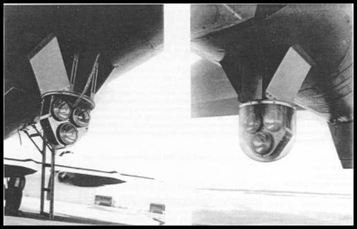
Photographs showing the high-intensity flashing beacon, installed in place of the lower aft gun turret just forward of the tail skid, used in LOLA observations.
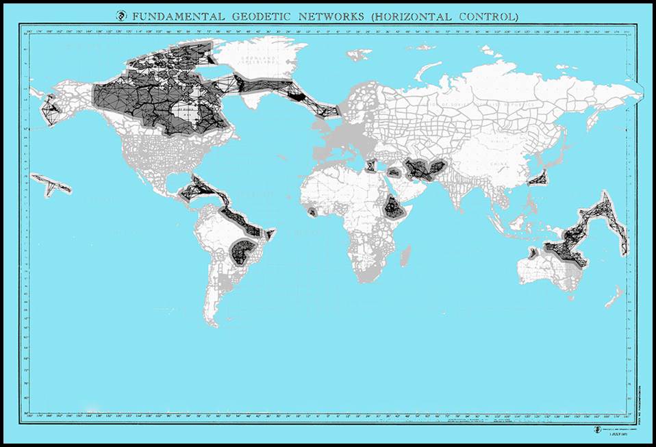
Map showing major Shoran, Hiran and Shiran networks along with world triangulation and traverse schemes, after Rankin (2016) modified from US Army Topographic Command July 1971.
Note the networks in Western Australia, Queensland, and the Great Barrier Reef, Australia plus some in Canada were acquired using Aerodist.
Major Hiran networks (refer map above) included :
Caribbean Island Tie : Between 1951 and 1953, Hiran was used on a network which tied Florida with the Bahama Islands, Cuba, Haiti, Dominican Republic, and Puerto Rico south to Trinidad and South America. This work provided a tie between North and South America independent of the conventional overland tie through Central America. In addition, the network allowed the Inter-American Geodetic Survey (IAGS) to extend the North American Datum 1927 (NAD 27) into Cuba. This project determined that Grand Bahama Island, lying 60 miles off the Florida coast, was then shown on charts six miles out of position. Cuba was also misplotted by 0.6 miles. The positions of other islands were also erroneously represented on the charts. After the network was adjusted on the North American Datum 1927 an overall accuracy of 1: 113 000 was quoted as being achieved. A map showing the northern section of this work is at Annexure B, Map B2.
Eastern Mediterranean Tie : In 1952 the United States Army Map Service initiated a project for a geodetic connection between North Africa and the Greek triangulation in the Aegean Sea. The network specifically tied the islands of Crete and Rhodes with Libya and Egypt. The Eastern Mediterranean Tie strengthened the existing triangulation around the Eastern Mediterranean, then being readjusted, by a direct tie with the adjusted European net across the Mediterranean Sea. The connection was carried out in the summer of 1953 by the United States Air Force in cooperation with the Greek Army Geographical Service and the Survey of Egypt. A map showing this work is at Annexure B, Map B3.
North Sea Tie : Also in 1952, and again at the request of the Army Map Service, and in cooperation with the Ordnance Survey of Great Britain and the Geografiske Oppmaling of Norway, a direct connection between the triangulation of the British Isles off Scotland and the Shetland Islands, and that of Norway was made. The North Sea Tie closed the loop of existing triangulation around the North Sea. A map showing this work is at Annexure B, Map B4.
North Atlantic Tie : Completed in 1956, this network connected the North American Datum 1927 to the European Datum, from Canada to Scotland and Norway by way of Greenland, Iceland and Baffin Island.
Mid-Pacific Survey : In late 1958, a Hiran network was completed connecting Wake Island, Kwajalein and Eniwetok Atolls, and the Taongi Islands.
Cuba-Central America Tie : Also known as the Yucatan Tie, this survey was completed by the close of 1959.
Japan-Taiwan Tie : Between October 1959 and February 1960, a Hiran survey stretching from Japan south through the Ryukyus island chain to Okinawa, and then westward to Taiwan, was completed. This network established a geodetic tie between the datum at Tokyo (Japan) and the Koshizan datum of Taiwan.
Brazil-Venezuela Tie : During 1960, a precise geodetic tie across a large gap in the existing ground triangulation of northeastern South America was made. The region was a strip 1,700 miles long and 500 miles wide across the countries of Venezuela, British Guiana, Surinam, French Guiana and Brazil. Within this region lay almost inaccessible terrain because of the mouths of the Amazon and Orinoco Rivers, rainforest, jungle, savannah, and mountains.
Eastern Pacific Tie : The Hawaiian Archipelago, along with Midway and Johnston Islands were connected by Hiran and established on a common datum. This long narrow network had no connection with any existing datum, so it was necessary to ascertain the astronomic azimuth of 16 of its lines. Azimuth of 11 of these lines were accomplished by LOLA, with the azimuth of the remaining 5 lines determined by traditional methods. The survey was completed by 30 June 1962.
Southwest Pacific Survey : This extensive Hiran survey was undertaken between 1962 and 1964 and tied Australia with Papua New Guinea, the Bismarck Archipelago, the Caroline and Marshall Islands, the Gilberts (Kiribati) and the Ellice (Tuvalu) Islands, and Fiji. This survey, also known as project AF60-13, included some of the longest Hiran lines ever measured, with the longest and Hiran record being 576 miles (930 kilometres). To achieve these long distances, the Boeing RB-50 aircraft as shown in the photograph below, had to get special approval to exceed their operating limit of 37 000 feet and struggle to 43 000 feet. A map showing this work is at Annexure B, Map B5.
In addition to the countries listed above, Hiran Aerial Survey Teams also operated in Spain, Ecuador, Colombia, Peru, and Vietnam.
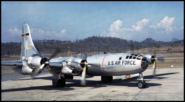
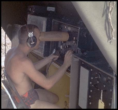
Left is a Boeing RB-50 used on the Southwest Pacific Survey at Jackson Field, Port Moresby PNG in 1963; Right, is a Hiran ground station operator surrounded by the necessary measuring and communications devices (Courtesy of George Jeff Flemming).
Shiran
A further development of Shoran/Hiran in 1965 was SHIRAN (S-band Hiran). Initiated in 1962 the AN/USQ-32 system, commonly referred to as Shiran, was developed by the Cubic Corporation of San Diego, California, under direction of the Systems Engineering Group of Dayton, Ohio.
Unlike Hiran’s pulsed emissions, Shiran emitted a continuous wave from the airborne master unit at an amplitude modulated frequency of 3.312 GHz (S-band). Four ground responders were sequentially interrogated in turn up to 10 times/second. The amplitude modulation at four frequencies, 663, 41.4, 2.6kHz and 162Hz, allowed the distances to each of the ground responders to be measured at four different wavelengths. Thus unambiguous range measurements of up to 500 nautical miles (900 kilometres) could be resolved to 0.725 feet (0.2 metres). The measurement data were recorded on magnetic tape and processed by an electronic computer which could be installed on the airborne platform itself. The system was capable of generating, in near real-time, the coordinates of one of the ground stations, provided the coordinates of the other three ground stations were already known. Positioning capability of the system was shown to be around 10 feet (4 metres).
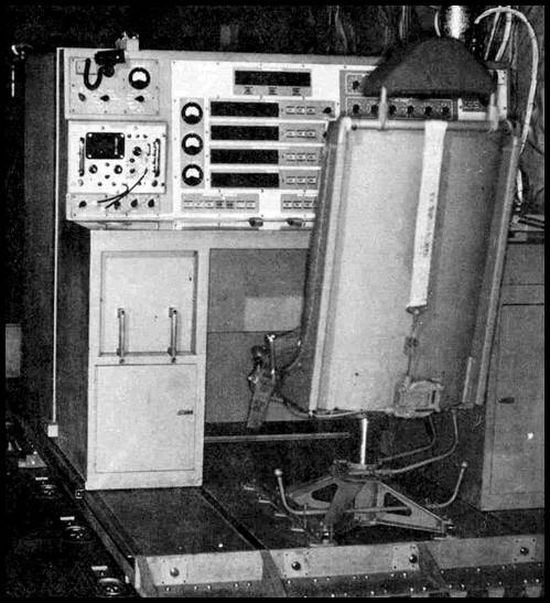
Shiran AN/USQ32 aircraft integrator console.
In addition to its four station ranging capability, the Shiran system had a simple calibration feature. Calibration of the airborne subsystem was accomplished at the press of a button whereby the integrated test oscillator measured the phase delay and placed it in memory. This phase delay was then automatically subtracted from each subsequent range measurement. System calibration was accomplished within ten seconds. Calibration could also be checked at any time to guard against drift. The 1964 paper, SHIRAN - AN/USQ-32 Microwave Geodetic Survey System by Bush and Pappas, provides greater detail.
The positional accuracy provided by the AN/USQ-32, Shiran system saw it incorporated into the Kollsman Instrument Corporation’s, Aerial Electro-Photo Mapping System. The initial concept was described in Kingsley’s 1964 paper, A New Technique for Aerial Mapping. Boeing KC-135 aircraft, conceived and designed as a high speed, high altitude stable platform for air refuelling missions, retained its centre of gravity throughout refuelling operations. As the tanker’s own fuel was below the cargo floor an area the size of a bowling alley was available to accommodate multiple cameras, electronic survey equipment, etc. The sophisticated auto pilot complimented the stability characteristics of the aircraft, maintaining it rigidly in space as a firm stable platform ideal for aerial mapping operations. It was expected that this new system, in addition to mapping photography, would acquire the control data required for large scale (1: 50 000) maps.
The Kollsman Aerial Electro-Photo Mapping System, designated AN/USQ-28, was considered the most sophisticated survey/mapping system ever built, and operated in the late 1960s and early 1970s. Four such systems were installed in Boeing Stratolifter RC-135A aircraft, becoming operational in 1966. The Boeing Stratolifter RC-135A was developed from the KC-135A Stratotanker, both of which were derived from the Boeing 707 prototype. The RC-135A could cruise at 855 kilometres/hour at an altitude of 10 700 metres for 7 400 kilometres. The four electro-photo mapping platforms were utilised briefly by the Air Photographic & Charting Service, based at Turner Air Force Base, Georgia and later at Forbes Air Force Base, Kansas as part of the 1370th Photographic Mapping Wing.
The 1964 paper by Di Carlo and Grady, Mapping and Survey System Geodetic, AN/USQ-28, detailed the system which included :
|
an advanced design mapping camera with a recorded thirty arc second verticality; |
|
|
- |
an extremely precise inertial navigation system; |
|
- |
distance measuring equipment with increased range and accuracy (Shiran); |
|
- |
a terrain profile measuring sensor with increased range; |
|
- |
advanced design navigation and photographic optical viewfinders; and |
|
- |
a light source with variable intensity light for long line azimuth (LOLA) measurements. |
Apart from the aerial photographs, all supporting data was recorded on magnetic tape for direct input into a ground digital computer for accurate and rapid data editing and reduction.
The system was designed to have the following capabilities.
|
Capability |
Description |
|
1 |
Acquire precision aerial photography whereby the aircraft flies long parallel flight lines with control of the forward overlap and sidelap of the photography to a high degree of accuracy, plus recording all supporting data.
|
|
2 |
Aerial electronic surveying : geodetic control networks by trilateration where after each line in the network is measured, a network adjustment computation provides the most probable position for each station; or line measurements by a technique known as "line crossing" by flying the aircraft across an imaginary line connecting two non-intervisible, ground stations while simultaneously recording the distance to each station and other applicable auxiliary data.
|
|
3 |
Acquire electronically positioned mapping photography by, in addition to Capability 1 above, record the distance to several Shiran ground transponders at the instant that the aerial mapping film is exposed. The location of the point directly beneath the aircraft (the nadir point), relative to the ground transponders is computed. The photograph can then be placed in its proper position on the earth's surface. The accuracy of these nadir points are within twenty-four feet (8 metres) with 90% probability as referred to the ground stations from which they were established.
|
|
4 |
Acquire horizontal control point photography by using three Shiran transponders to position mapping camera photography obtained with a recorded verticality of thirty arc seconds, and thus co-ordinate prominent features on the face of the earth within a probable error of 15 feet (5 metres). This capability reduces the need for ground survey parties to provide ground control to support aerial mapping photography.
|
|
5 |
Terrain Profile Recording to generate the terrain profile along the flight track of the aircraft. The terrain data provides vertical control for the mapping photography. This function is normally accomplished in conjunction with electronically positioned aerial mapping photography, horizontal control photography and precise aerial mapping photography.
|
|
6 |
Long line azimuth (LOLA) determination where trilateration is unsuitable, the measurement of geodetic angular information, to the aircraft mounted light source, in addition to distance is a necessity.
|
Such capabilities theoretically meant that an airborne survey could be completed for an area about the size of Tasmania in a couple of weeks.
Shiran did not replace Hiran completely, but was used on a 1970 survey of the interior of Brazil.
During 1972, however, the four RC-135A photomapping aircraft were converted to other uses as the cost of upkeep for photomapping could no longer be justified. The United States Air Force finally deactivated its Hiran/Shiran surveying capability in 1974 when satellite positioning became available.
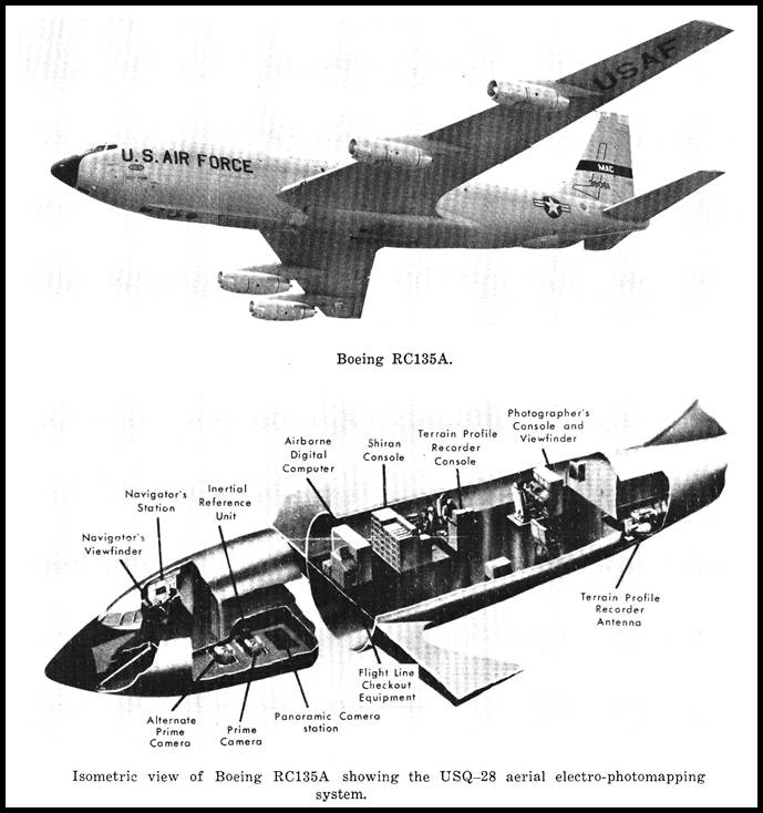
Shiran AN/USQ-32 system, forming part of the AN/USQ 28 system, installed in a Boeing Stratolifter RC-135A.
Shoran in Australia
Formation of the National Mapping Council (NMC) in 1945 was followed by the Council’s first meeting in the September that year. The chair for the meeting was Frederick Marshall Johnston, then Director of National Mapping as well as Commonwealth Surveyor General and the Commonwealth’s Chief Property Officer. To assist Johnston with the National Mapping role, Bruce Philip Lambert was appointed Deputy Director of National Mapping in late 1946.
An early priority for the NMC was a national geodetic survey. However, Australia’s overall size and the vast sparsely populated regions to be surveyed meant that much of the mainland would be without geodetic survey control for some time. Airborne EDM was considered as a potential means of rapidly extending control from the proposed geodetic survey. An airborne EDM system would allow connection to areas where more intensive surveys would be required and at the same time permit a series of widely scattered survey points to be fixed. This national framework would form the basis for controlling the surveys for any areas of isolated development.
Almost immediately after his 1946 appointment as Deputy Director of National Mapping, Bruce Lambert travelled to the United Kingdom, Canada and the United States to see how their national mapping agencies operated. He also wanted to gain an understanding of their use of radar for geodetic survey. This interest in the use of radar based EDM for surveying, mapping and aerial photography was not limited to the National Mapping Section of the Department of Interior where Lambert was based. Then Director of Military Survey, Colonel Lawrence Fitzgerald, explained to the congress of the Australian and New Zealand Association for the Advancement of Science held in Adelaide in 1946, that considerable interest was being taken in recent developments in the application of radar to surveying. Such was the Survey Corps interest that two of its officers, Major HA Johnson (who was later to join National Mapping) and Lieutenant FD Buckland, were sent to England at the end of that year. Their task was the specific study of radar aids to mapping. While overseas during 1947, the two Army officers also went to Kenya in July for two months to observe, the previously described, radar-controlled air survey task being performed by the British. The RAAF was also interested in becoming involved with the new technology. Around this time, two of its officers were also sent to England to gain maximum knowledge of the new radar systems.
At least one driver behind these study tours appears to have been resolutions adopted by the Commonwealth Survey Committee (CSC). Although formed in 1935 as the government’s response for a coordinating body to control now disparate Australian survey and mapping activities, the CSC did not really meet, due to the war, until August 1944. The CSC was chaired by the Commonwealth Surveyor General, with representatives of the three Defence services (Navy, Army and Air Force). Coordination with the States was achieved through the Commonwealth Surveyor General. For some years, the CSC and the NMC operated in parallel before the CSC was finally abolished. CSC resolutions, numbers 15 and 33 were likely adopted at 1945 meetings of the CSC and read :
No.15 - That this Committee, having heard the views of Dr E.G. Bowen on the application of radar to surveying, inform the C.S.I.R.O. of the Committee's keen interest in the subject and recommend for favourable consideration by the Council a proposal that further research be made into the design and use of radar equipment suited for survey purposes under Australian conditions [Dr Edward George (Taffy) Bowen (1911-1991), was then Chief, Radiophysics Division of CSIRO (Bhathal, 2014)].
No.33 - That this Committee notes the development of the application of Radar to surveying, particularly with reference to aerial photography, and considers that the conditions existing in Australia and the Territories warrant the introduction of this equipment at the earliest possible moment, and recommends that the R.A.A.F. adopt the Radar Control method of photographic air surveys, and be responsible for selection and procurement of the most suitable air and ground equipment, and operation and maintenance of this equipment.
After returning from his four-month overseas study tour, Lambert was upbeat about the use of radar for mapping. In Canberra on Thursday 17 October 1946, he gave an address based on observations made during his overseas trip. Lambert’s address was titled: Modern Developments in Surveying and Mapping. It was presented at the closing of the conference on Mapping and Survey Problems. Conference attendees included Surveyors General from all states and the Commonwealth Surveyor General. Lambert’s address was reported on page 4 of the next day’s Canberra Times under the headline RADAR TO SPEED COMPLETE MAP OF AUSTRALIA. In the report, Lambert is quoted as saying war-time developments of radar and radio will prove invaluable to the future when carrying out national survey and mapping schemes and should be of great assistance in extending the small area which so far has been adequately mapped in Australia. The complete article is shown below.
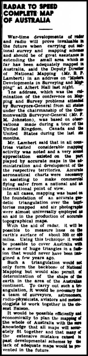
Article from page 4 of The Canberra Times of Friday, 18 October 1946.
At its third meeting on Monday 14 October 1946, the NMC resolved to appoint the advisory committee on the Radar Triangulation of Australia. The committee under the chairmanship of Dr Richard van der Riet Woolley, Commonwealth Astronomer, comprised Dr Joseph Lade Pawsey and Dr Jack Hobart Piddington of the Radiophysics Division of CSIRO, Colonel Lawrence Fitzgerald, Director of Military Survey, and Mr Bruce Philip Lambert, Deputy Director of National Mapping. Their brief was to advise on the practicability of using radar to create a framework of accurately surveyed points over the whole of mainland Australia. Such a framework would enable all survey and mapping activities to be coordinated on a national basis. This committee met at the Commonwealth Observatory, Mt Stromlo on Tuesday 17 December 1946, and discussed the problems involved and arranged for the necessary investigations to be undertaken.
Over a year later on Monday 2 February 1948, Fred Johnston the then Commonwealth Surveyor General and Director of National Mapping, addressed the Rotary Club of Canberra. His address was reported on page 2 of the next day’s edition of The Canberra Times under the headline RADAR MAPPING PLANNED FOR AUSTRALIA. Johnston was quoted as saying new equipment is on order by the Commonwealth Government and, when it arrives, mapping by radar will become an established fact in Australia…the use of radar for mapping purposes was availed of during the war years overseas and it provided unbounded possibilities. While it was not entirely clear, most likely the equipment Johnston had talked of was the Radio Corporation of America (RCA) Shoran aircraft set AN/APN-3 and two ground responder sets AN/CPN-2. This equipment was used to evaluate Shoran for obtaining Australian survey and mapping control. Please refer to Annexure C for the details of the equipment.

1949 photograph of operator with CSIRO with a Radio Corporation of America (RCA) Shoran aircraft T-11/APN-3 transmitter in Douglas Dakota C47B aircraft, with explanatory diagram.
Subsequent to the NMC establishing the advisory committee on the Radar Triangulation of Australia, a subcommittee of the NMC was tasked with assessing whether Shoran would provide a means of accelerating the Australian mapping program. This subcommittee arranged with CSIRO to carry out tests using Shoran. Radar expert, John James Jack Warner of the Division of Radiophysics carried out and reported on the Shoran testing. Warner adopted a methodology briefly described by Edward George Bowen, then Chief of the Radiophysics Division of CSIRO, in his 1947 paper Radar Aids to Surveying.
The criterion for acceptance of Shoran for airborne trilateration was a line measurement accuracy in the vicinity of 1: 100 000 or 1 metre in 100 kilometres. As it was already known that the best accuracy was only around 1: 50 000, extracting a fifty percent improvement from the system was a big ask. The line crossing technique was used with multiple line crossings at varying altitudes.
A suitable braced quadrilateral, wherein all six distances were already known from previous, high accuracy, ground survey, was selected in New South Wales. The quadrilateral had its vertices near Condobolin, Tamworth, Sydney and Canberra, as shown in the map below. The lines to be measured ranged from 158 to 311 miles (250 to 500 kilometres).
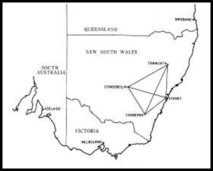
Map showing the relationship of the Shoran test quadrilateral’s vertices near Condobolin, Tamworth, Sydney and Canberra.
The testing was documented in Warner (1950) which recorded that the airborne equipment, designated Radio Set AN/APN-3, was installed in a Douglas Dakota C47B aircraft, flown and maintained by the Royal Australian Air Force’s, Aircraft Research and Development Unit (ARDU).
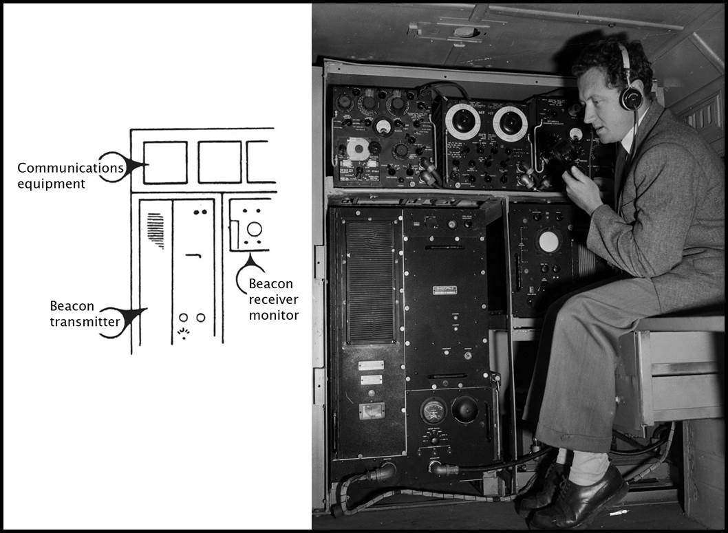
Photograph of a Shoran ground station transmitter, T-12/CPN-2, and monitor ID-18/CPN-2, with explanatory diagram.
Additional instruments were added in the form of a radar altimeter and equipment capable of measuring meteorological parameters in flight. A Pilot's Direction Indicator was a late addition. It consisted of a pair of counters, one recording the sum of the two air-ground distances, and the other the difference. By flying the aircraft so that the difference counter remained constant the aircraft’s track was suitable for line crossing. Since the sum of the two distances was a minimum at the crossing point and increased on either side, the sum counter was used to indicate to the pilot that he had flown far enough on either side of the line to permit a satisfactory record of the line crossing to be obtained. This device also enabled operations to be carried out when the ground below was obscured by cloud.
The ground station responders, designated Radio Set AN/CPN-2, were initially installed in trailers with one subsequently installed in the back of a covered truck. The photograph below, is understood to show one of the ground station equipment trailers with its aerial in the stowed position; the antenna could be raised for measuring operations.
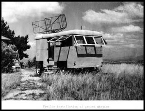
The line measuring operations required 18 months to complete with a total of more than 150 line crossing measurements taken over the six lines. Overall an accuracy of about 7 parts in 100 000 or some 20 metres over a 300 kilometre line was achieved. This accuracy equates to about 1: 15 000 with even the best result only 1: 77 000. An individual measurement on any one line was considered to be within about 7 metres.
This Australian test gave accuracy results comparable with those obtained elsewhere and reinforced the fact that Shoran’s systematic equipment errors proved the main limiting factor in obtaining higher accuracy. Warner suggested that by suitable modification to the equipment, in particular to the receivers, the signal intensity error could be reduced [and] the overall accuracy of the technique would improve to about 2 parts in 100,000. An improvement on this latter figure would be impossible without extensive improvements to the radar equipment, particularly to the phase shifting goniometers and the display. In addition, a thorough investigation of problems of atmospheric refraction would be necessary. Some similar such improvements to Shoran had already been undertaken by the Americans to develop their Hiran system.
Rimington and others (1954) stated whilst these [Shoran] tests were being carried out, a representative of the National Mapping Office acted as an observer, to try and gather some idea of the economics of the whole problem. The facts that he gathered in regard to the operation of the equipment were such that the subcommittee on Radar could not recommend the method as an economic proposition. It was felt by the subcommittee that the demands on money and manpower required to use Shoran for mapping purposes would be beyond the very tiny resources of the existing National Mapping Office.
Lines (1992) wrote that the ultimate decision to abandon Shoran for geodetic work came in 1949. The reasoning behind the decision was that :
|
- |
the required accuracy was not attainable; |
|
- |
extending radar trilateration over long distances into unsurveyed inland Australia without some intermediate or end geodetic based check or azimuth control, was an unsound survey technique; |
|
- |
the ground equipment was relatively bulky and heavy, and required heavy vehicle transport limiting the locations on where it could best be located; |
|
- |
costs were uncertain, and beyond the financial and personnel resources then available to the National Mapping organisation. |
While a pragmatic decision given the facts, it no doubt came as a blow to Lambert and others who until now had been proclaiming the benefits of radar based airborne EDM.
Rimington (1960) noted that at about this time Dr Erik Osten Bergstrand had demonstrated his first models of the Geodimeter, and it was decided to acquire and test a production model of the instrument before finally deciding on a type of electronic distance measuring equipment for use in Australia. A unit of the equipment was obtained in 1953 and thoroughly tested with results that have had great significance. The results of these tests, which agreed consistently with those carried out in other countries of the world, established that electronic measurement of the lengths of normal geodetic lines was not only practicable but also had a phenomenal degree of accuracy. It was considered a remarkable advance over Shoran airborne electronic measuring equipment, which relies on extreme length of line (up to 400 miles) to achieve its fractional accuracy. It was established that the Geodimeter Type NASM-1 could measure distances with a limiting error of ±0.08 feet (approximately ±1 inch or ±24 millimetres). Here then was a system that could eliminate the time consuming base line and its associated network, substituting the direct measurement of a single side of triangulation for all such base lines. The example below, shows the complexity of a traditional National Mapping base net near Broken Hill in 1954. The red line North Base-South Base was to be measured to a high precision with a special steel band. Then by observing the internal angles of the blue network of triangles the length of the major triangulation line Moorkaie-Sundown could then be derived to an equivalent accuracy. The timely introduction of the Geodimeter meant that the green line Twenty Mile-Felspar could now be measured rather than this complex base net thereby achieving the same outcome in days rather than weeks.
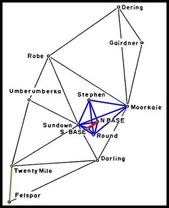
Example of a traditional National Mapping base net near Broken Hill in 1954.
The red line North Base-South Base was to be measured to a high precision with a special steel band. Instead the green line Twenty Mile-Felspar was measured by Geodimeter EDM.
Control for Australian mapping now followed a more traditional route of geodetic triangulation and flexible, priority based, position-fixing by astronomical observation. History shows that other interested members of the committees likely took note of the outcome of the Shoran testing. Even the Royal Australian Survey Corps, who were also initially interested in airborne radar EDM and whose resources were greater than National Mappings’, continued with traditional survey and mapping methods.
Nevertheless, in late 1952, the first Australian application of Shoran to control mapping was for a project in the Rum Jungle area of the Northern Territory. Accurate planimetric maps were required to serve as a base for prospectors' charts, at a scale of one mile to an inch, showing radioactive anomalies obtained from airborne scintillometer surveys conducted by the Bureau of Mineral Resources. The West Australian newspaper of Thursday 31 July 1952, announced on page 7, Uranium Field to Be Air-Plotted…The Rum Jungle uranium field in the Northern Territory is to be plotted soon from the air by geophysicists of the Bureau of Mineral Resources. A Dakota aircraft, fitted with equipment recently delivered from Canada and America, will be used…the expedition will have its headquarters at Darwin and the aircraft will fly courses that permit continuous readings along lines half a mile apart. To ensure accuracy, the pilot (Capt. lvo Duffell, of Trans-Australia Airlines), will navigate by an electronic aid, developed during the war, called "shoran". From this letter of 18 February 1949 to National Mapping from the then Zinc Corporation Limited, it appears that Natmap had had experience with astrofixing the positions of Shoran ground stations from as early as 1949.
For the Rum Jungle surveys, the airborne equipment, including the Shoran AN/APN-3, was carried by the Bureau of Mineral Resources’ Dakota aircraft VH-BUR. Two Shoran responder, vehicle-borne units (AN/CPN-2) provided fixed ground control. The Shoran units were loaned by the Radiophysics Laboratory of CSIRO, Sydney and were most probably the same units as used on the 1949 evaluation described above. Before leaving for the Northern Territory the equipment was tested around Melbourne. In the Northern Territory the vehicle-borne responders were set up near Mt Peel and Mt Tolmer, a distance of 28.26 miles (45.5 kilometres) apart and about twenty miles or thirty kilometres north-west and south-west, respectively, of the then Rum Jungle mining camp. This camp was about 10 kilometres north of the present day town of Batchelor. Please refer to the map below.
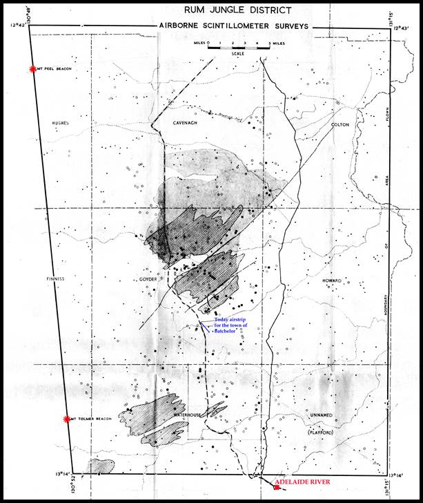
Map of 1952 Rum Jungle survey area showing locations of Mt Peel and Mt Tolmer Shoran responders in relation to Adelaide River, the then nearest town. The airstrip marked in blue is today used to service the town of Batchelor situated just to its north. The then Rum Jungle mining camp was about 10 kilometres north of the airstrip.
From BMR’s perspective they were happy with the outcome of the survey and stated with the Shoran equipment it is possible to pin-point radio-active areas sufficiently accurately to enable ground parties to locate them. This reduces the amount of ground surveying to a minimum and so speeds up greatly the rate at which an area can be investigated. The Melbourne Age newspaper reported on the spectacular results of the Bureau of Mineral Resources’ surveys. The Bureau, who had used Shoran positioning during their 1953 airborne surveys, and had been successful in their search for oil in Gippsland, iron on the Eyre Peninsula, and copper on the Yorke Peninsula.
From National Mapping’s perspective the Rum Jungle survey results were not so exciting. The details are in a 1954 paper by Rimington etal, Application of Shoran to Australian Mapping. A major failure of the project was that the F24 camera installed in the aircraft to provide positioning photography was subject to aircraft movement, tip and tilt, thus the air position coordinates provided by Shoran could not be accurately transferred to the ground. The Shoran system had not been able to meet the Australian geodetic specifications. However, in that era the radar based technology was still of great interest. If pursued, technical advances might soon make radar useful to surveying and mapping Australia’s vast landmass. The extent of this interest was evidenced by the terms of reference for the Brown report containing a specific requirement that Brown’s investigation: should cover the following technical matters…the implications of the adoption of radar triangulation on the national system.
Major General Reginald Llewelyn Brown, then Director General Ordnance Survey of Great Britain, finished his report to the Minister for the Department of the Army in December 1951. At the invitation of Australian authorities, Brown had visited Australia in early 1951. He had met with State and Federal mapping agencies to gain the information vital for him to formulate the advice required under his terms of reference.
Regarding radar, Brown covered the uses of radar for surveying in war; the value of radar in the geodetic framework, he cited Canada’s Shoran experience and supported Lambert’s 1946 view detailed above. Brown also covered air photography and radar techniques. Brown concluded: it does not seem likely that radar triangulation will ever be able to replace geodetic triangulation altogether…the present radar technique is unable to measure short distance. Furthermore, radar cannot be related with sufficient accuracy to astronomical observations for azimuth. It should not therefore be allowed to delay any projects for geodetic triangulation. In his recommendations to the Minister, Brown stated experience in radar triangulations be gained within Australian territory as soon as possible and that geodetic triangulation be not delayed on that account. Hindsight shows that, as discussed further on in this paper, radar technology was the way forward as within 5 years highly portable terrestrial EDM was available followed by airborne EDM about 5 years after that.
Following his four year term as Director General of Ordnance Survey, Brown retired in 1953. In retirement, Brown consulted to Spartan Air Services of Canada for their work in Europe and the Middle East which included aerial photography, magnetometer, scintillometer, electromagnetic, Shoran and Airborne Profile Recorder surveys. When, in 1963, Spartan bought an interest in Meridian Airmaps Limited, Brown was appointed Chairman. In 1973, Meridian repurchased the Spartan interests and Brown continued as Chairman of the company until his death in 1983.
Based on the results of the Bureau of Mineral Resources’ 1952 use of Shoran, the technology was adopted for positioning in resource exploration. The Bureau of Mineral Resources used advanced Shoran (AN/APN-84 and AN/CPN-2A). These were later models than those used for the 1949 and 1952 work. The advanced Shoran models became available in the mid 1950s. The AN/APN-84 master station was fitted in the aircraft and three AN/CPN-2A responder stations were fitted into Morris Commercial, four wheel drive trucks. The aircraft master interrogated two ground responders at a time to give a continuous fix of the aircraft's position. The ground responder sets were positioned as close as possible to previously fixed survey stations. While two of the ground responders were in operation the third could be repositioned, permitting almost continuous flying operations.
The Bureau used this system for positioning in the offshore Perth Basin in 1957, Carnarvon Basin in 1956 and 1957, Broken Hill district during 1957 and 1959, the Bonaparte Gulf Basin in 1958 and Tennant Creek Mineral Field in 1960. Later in 1961, Haematite Explorations Pty Ltd used Shoran as a navigational aid for the offshore survey of the Bass Strait as did the Texaco Overseas Petroleum Company in 1969 in the Papuan Basin in the Torres Strait. In 1968, the Western Geophysical Company of America was the prime contractor and operator for Esso Standard Oil (Australia) Limited (the phonetic version of the initials of Standard Oil i.e. SO or Esso and the American trade name for ExxonMobil). Offshore Navigation Incorporated was subcontracted to provide survey control using Shoran for the marine survey of the Otway Basin of south-west Victoria. Offshore Navigation Incorporated also operated off shore in the north-west of Western Australia around 1965. By the late 1960s, however, more sophisticated and accurate methods of navigation/position fixing had been introduced.
Natmap Aerodist line measuring operations for Block 36 took place in 1973. This work extended survey control offshore around Onslow. On Tuesday 28 August 1973 an existing station Shoran 11 was occupied and intersected by lines from mainland stations Onslow (R299) and Minnie (KAP8). Station Shoran 11 was also spot photographed from 3 000 feet. None of the readily available information mentions station Shoran 11 but it was probably established for exploration activities. National Archives Australia hold a series of records in Perth from 1966, titled Survey and mapping - Shoran Survey - Onslow - Barrow Island - Station notes. The Recording Agency is listed as 5 Field Survey Squadron, Australian Army, and the Controlling Agency, Defence Corporate Services and Infrastructure Centre, Western Australia. Station Shoran 11 could thus have been established by the Squadron.
National Archives Australia also holds records indicating that National Mapping fixed points for later occupation by the Bureau of Mineral Resources Shoran ground responders. The points were in the Rum Jungle, Tennant Creek and Broken Hill areas. In his 1979 paper, The Division of National Mapping’s Part in the Geodetic Survey of Australia, Ford makes mention of the Eyre Peninsula, Rum Jungle and Broken Hill surveys also being required by the Bureau.
By the mid 1980s, the use of terrestrial or airborne radar EDM systems in Australia for surveying and mapping had already passed into history by some ten years. It was therefore surprising to find Bowen’s 1987 description of events as is reproduced at Annexure A below. Suffice it to say that Bowen’s account reflects that described in his 1947 paper rather than what actually happened, as was detailed above!
Horizontal Mapping Control from Fully Oriented Aerial Photographs
A persistent vision in National Mapping, and world wide to a large extent, was to provide horizontal mapping control without having to have a survey party occupy the actual control points. The theory ran that by taking aerial photographs of the region where the mapping control was required, accurate coordinates of feature(s) in the photoframes could be calculated. However, the coordinates of the positioning camera platform at time of exposure were required as was the camera’s orientation, tip and tilt, as no aerial photograph was truly vertical. As was found in the 1953 Shoran based work in the Northern Territory, described above, the major obstacle lay in determining the positioning camera’s orientation at the time of exposure.
McLean’s (2015), The Aerodist Years described the next attempt using Aerodist phototrilateration. Even with the addition of a special horizon camera, the tips and tilts of the then Vinten positioning camera could not be determined accurately enough to provide suitable ground control coordinates.
Around 1975 came an internal Natmap Proposal for Linear Edge Control of Photogrammetric Blocks, please refer to Annexure D below. The proposed method to obtain mapping control by photographic means was never implemented. The proposal document also mentioned another project that was to provide the tip and tilt of an aerial survey camera at time of exposure, namely the Camera Attitude Indicator (CAI).
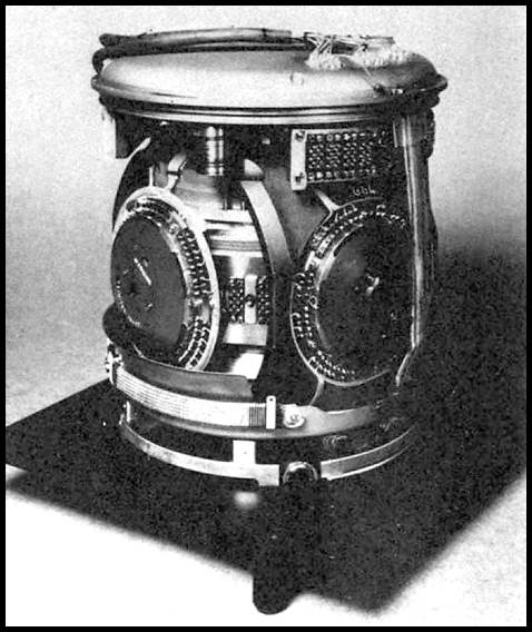
Inertial platform by Ferranti after Brinker and Minnick (1987).
According to Natmap Assistant Director, Lines, in his 1975 paper, Inertial Platform and Attitude Indicator for an Airborne Photogrammetric Camera, the idea emerged from Canadian and American developments described in Zarzycki (1964) and Bush and Pappas (1964) and Di Carlo and Eakin (1964). The cost and complexity of these systems, especially the Kollsman system discussed above, was prohibitive to Natmap but technology had moved on and devices had become smaller and cheaper. Initially inertial navigation systems incorporating very precise gyroscopes, which might have had the capability of achieving acceptable accuracies in the measurement of pitch and roll at the instant of exposure of an aerial camera, were explored by the Division of National Mapping and the then Department of Supply, Australian Defence Scientific Service, Weapons Research Establishment (WRE) at Salisbury, South Australia (through the development and operation of the Laser Terrain Profiler, Natmap and WRE already had a strong working relationship). In mid 1971, however, gyro-accelerometer (inertial) solutions emerged as having the required accuracy of 10 arc minutes being maintained over a period of one hour.
An inertial system contained two types of components, accelerometers and gyroscopes, which sensed motion. In principle, as matter resists changes to its motion it has inertia. Operationally, an accelerometer measures acceleration, integrating once to give a measure of velocity and twice to give a measure of distance travelled. The direction along which an accelerometer measured was kept fixed in space by gyroscopes which provided a stable attitude reference. The accelerometers were thus fixed and oriented relative to each other on a rigid platform which in turn was mounted on gimbals. Thus this mechanism was isolated from any changes in attitude as it was being transported. Any platform rotations about three perpendicular axes were sensed by the gyroscopes causing motors acting about the gimbal axes to respond. The whole configuration was termed an inertial platform. Please refer to the photograph above.
Ferranti Ltd., UK, received the Queen's Award to Industry in 1967 for producing a small inertial platform weighing about 10 kilograms around a quarter of the weight of its earlier model. The Ferranti lightweight platform, was designed and manufactured at Ferranti's Edinburgh laboratories, Scotland, as a four gimbal, fully acrobatic, lightweight platform, primarily for use in aircraft, but suitable for any system requiring a high accuracy inertial reference.
The Ferranti lightweight platform was installed in the Hawker Siddeley P1127 vertical take off and landing aircraft, the Harrier. A prototype Aérospatiale/ British Aircraft Corporation (BAC) Concorde also contained the Ferranti platform but the platforms used in operational Concordes came from another supplier. Ferranti systems were also produced for the European Launcher Development Organisation (ELDO) and the Black Arrow program. Black Arrow, officially capitalised BLACK ARROW, was a British satellite carrier rocket developed during the 1960s. Of its four launches, between 1969 and 1971 from Woomera here in Australia, only the final launch was successful and inserted the Prospero satellite into low Earth orbit.
Arrangements were made with the Royal Aircraft Establishment, Farnborough, UK, and Ferranti Ltd., UK, for the supply and fabrication of a modified inertial platform, with Ferranti also to design and manufacture certain portions of the interface and recording components. Some of the instrumentation from Black Arrow was also to be incorporated into this new equipment. Ferranti also guaranteed that the attitude accuracy of the platform over a period of 6 hours from ground alignment would provide a maximum error (1 sigma) not exceeding 10 arc minutes for the recorded camera pitch and roll.
As part of the development, Natmap provided one of its Wild RC9 aerial survey cameras and funded WRE’s development costs. WRE’s role was to undertake the rigid mounting of the Ferranti platform to the RC9 camera body, converting and transmitting the coded pitch and roll data into the instrumentation panel of the RC9 camera so each exposed frame would contain the required angular data and the general assembly of all the equipment into a convenient, practical surveying system. A significant problem to be solved was that to load film into the RC9 camera, the magazine (which sat over the camera’s lens system and focal plane) had to be raised. Mounting the Ferranti system would prevent this function. WRE overcame the problem by adapting the film magazine to be side loading. The inertial platform was a sizeable piece of equipment in itself, having about the same footprint as the RC9 camera but was twice the height. When the Ferranti system was coupled with the RC9 camera it was a substantial and impressive looking device.
WRE gave the project the name TAVRS for Two Axis Vertical Reference System but after repeated problems on the bench the system failed. With satellite positioning technology emerging, the Camera Attitude Indicator (CAI)/TAVRS project was scrapped.
The idea that a GPS antenna might be attached to the nose and tail and each wing-tip of the photographic aircraft and thereby use that technology to measure the attitude of the aircraft at the time of photographic exposure was considered, but never eventuated either.
The South African Finale – the Aerodist System
From the mid 1950s and into the 1960s and later, EDM equipment for surveying and mapping emerged from South Africa. Just as a hundred years previously when the steel band had replaced the Gunter link chain for distance measuring, these instruments would have an even greater impact. No longer would waterways, swamp, forest, jungle, be a barrier to the survey or mapping team. Provided the two end points of a line were accessible and visible to each other, measurement between the two points was possible; what was in between was now largely immaterial.
The South African’s, to coin a phrase, killed two birds with one stone. Colonel Harry Baumann, then Director of the South African Trigonometrical Survey, wanted an EDM that was man-portable with a range out to 50 kilometres and an accuracy of not less than 1: 100 000. Bergstrand's Geodimeter was just too limited and too cumbersome having to be operated at night and from locations that were vehicle accessible because of the Geodimeter’s weight. The 1957 Tellurometer by Trevor Lloyd Wadley of the Telecommunications Research Laboratory was the solution.
The rapid emergence of the Tellurometer was the likely result of both Baumann and Wadley’s previous experience with radar systems. McLean (2015) recorded that Baumann was familiar with radar and with the existing Shoran and Hiran long range EDMs. McLean continued and also recorded that during World War II Wadley was initially part of the highly secret Special Signals Service in Johannesburg that worked on the development of radar systems. After specialised radar training in the United Kingdom, Wadley was posted to an operating radar station in the Middle East as the officer-in-charge. Here he worked successfully on improving the performance of the station’s equipment. Some of Wadley’s war time activities were of a secret nature and included working on the staff of British General Harold Alexander during his command of the Fifteenth Army Group for the invasion of southern Europe. It is highly probable that in addition to primary radar development, Wadley’s secret work involved secondary radar like Gee and possibly extended to the later Gee-H and even Shoran. Consequently, Wadley would have understood the intricate shortcomings of existing radar for use in surveying applications. His solution was to superimpose a low frequency wave on the signal using a precise method of phase comparison and creating the basis of the Tellurometer. Sales to Canada, Australia, the United States and numerous other countries resulted. The United States Army ordered several hundred Tellurometer instruments.
With intervisible lines now able to be measured almost without restriction, the focus turned to non-intervisible lines for which an airborne system would be required. The portability and range of the Tellurometer was the basis for the Aerodist (Aeroplane Distance) system. At the beginning of the 1960s, Canada and particularly Australia saw Aerodist as a viable system for use in their mapping programs and used the system with great success.
Between 1963 and 1974, the Division of National Mapping deployed an Aerodist MRC2 secondary radar system to provide horizontal control for the 1: 100 000 scale National Topographic Map Series. Nat Map used that system to obtain control over more than 50 per cent of mainland Australia and over some offshore areas. During the above period Nat Map’s Aerodist system measured some 3 020 lines to fix the positions of 485 survey control stations. Nat Map’s use of Aerodist is detailed in McLean’s 2015 work The Aerodist Years. McLean (2015) noted that the Royal Australian Survey Corps took delivery of an Aerodist MRC2 system in 1964. That Aerodist system was initially deployed in western Papua New Guinea. Subsequently RA Survey carried out Aerodist survey operations in Indonesia and in northern Australia including Cape York, Arnhem Land and the Kimberley. After the loss of its initial system in an aeroplane crash in November 1969, RA Survey updated its Aerodist system to the operationally more reliable computer assisted MRB3/201 equipment. The last field deployment of the Corps' Aerodist system was in 1975.
Concluding remarks
Essentially the Tellurometer and Aerodist was EDM at its peak. Other models and even other instruments came along afterwards using laser light rather than microwaves, solid state circuitry, digital readout and even automated data recording and processing. These were just improved versions of the basic concept.
In under twenty years, Aerodist technology had thus miniaturised every aspect of then airborne EDM for the measurement of non-intervisible lines of less than 350 kilometres. Unlike the earlier airborne EDM technologies, Aerodist was an economic option for National Mapping to employ for its 1: 100 000 scale topographic mapping control program. Ten years later as National Mapping was concluding its Aerodist surveys, positioning with the aid of artificial, earth orbiting satellites was already viable as a technology for providing mapping control. Thus, all airborne EDM became obsolete.
Acknowledgement
Thanks to Laurie McLean for his research contributions and valuable comments on the draft version.
References
Anonymous (1946), The Canberra Times, Friday 18 October 1946, page 4, accessed at : http://trove.nla.gov.au/ndp/del/article/2698075
Anonymous (1946), The Canberra Times, Thursday 19 December 1946, page 4, accessed at : http://trove.nla.gov.au/ndp/del/article/2703278
Anonymous (1947), The Sydney Morning Herald, Friday 24 January 1947, page 2, accessed at : http://trove.nla.gov.au/ndp/del/article/18018277
Anonymous (1947), Geraldton Guardian and Express, Tuesday 9 December 1947, page 4, accessed at : http://trove.nla.gov.au/ndp/del/article/67837979
Anonymous (1948), The Canberra Times, Tuesday 3 February 1948, page 2, accessed at : http://trove.nla.gov.au/ndp/del/article/2736600
Anonymous (1953), The Age from Melbourne, Friday 25 September 1953, page 2, accessed at : https://www.newspapers.com/newspage/123079447/
Anonymous (1984), In Memoriam R. Ll. Brown, The Photogrammetric Record, Vol.11, No.63, April 1984, pp.241-244. http://xnatmap.org/adnm/docs/bruno.pdf
Aerial Survey and Photomapping History (2015), Aerial Survey and Photomapping History, accessed at : http://www.1370th.org
Anderson, Wilmer C (1941), Final Measurements of the Velocity of Light, Journal of Optical Society of America, Vol.31, No.3, pp.187-197.
Aslakson, Carl Ingman (1949), Can the Velocity of Propagation of Radio Waves be Measured by Shoran?, Transactions American Geophysical Union, Vol.30, No.4, pp.475-487.
Aslakson, Carl Ingman (1951), New Determinations of the Velocity of Radio Waves. Transactions American Geophysical Union, Vol.32, No.6, pp.813-821.
Aslakson, Carl Ingman (1955), The Importance of Shoran Surveying, Transactions American Society of Civil Engineers, Vol.120, No.1, pp. 225-234.
Aslakson, Carl Ingman (1980), Earth Measurer, Excerpt from unpublished manuscript, http://www.history.noaa.gov/stories_tales/ak7.html
Aslakson, Carl Ingman and Rice, Donald A (1946), Use of Shoran in Geodetic Control, Transactions American Geophysical Union, Vol.27, pp.459-463.
Bergstrand, Erik Osten (1949), Measurement of Distances by High Frequency Light Signalling, Bulletin Geodesique, Vol.11, No.1, March 1949, pp.81-92.
Bergstrand, Erik Osten (1957), Some Recent Determinations of the Velocity of Light, N.1 del Supplemento al Vol.6, Serie X, del Nuovo Cimento, pp.224-231 (copy supplied by Oddbjörn Andersson, webpage from Kalmar, Sweden, in Swedish only www.storaalvaret.se).
Bjerhammar, Arne (1972), A Determination of the Velocity of Light using the Twin Superheterodyne Principle, Tellus, Vol.24, No.5, pp.481-495.
Black, Henry R (2015), The introduction of OBOE and H2S into RAF Bomber Command, accessed at : http://www.qsl.net/pe1ngz/stories/story-oboe-h2s.html
Blanchard, WF (2008), SONNE/CONSOL, in Hyperbolic Radionavigation Systems, compiled by Jerry Proc, 2015, accessed at : http://jproc.ca/hyperbolic/consol.html
Bomford, Guy (1971), Geodesy, 3rd Edn., Oxford at the Clarendon Press.
Bowen, Edward George (1947), Radar Aids to Surveying, Australian Geographer, Vol.5, No.5, pp.93-95.
Bowen, Edward George (Ed.)(1954), A Textbook Of Radar, 2nd Edn., Staff of the Radiophysics Laboratory CSIRO Australia, Cambridge at the University Press.
Bowen, Edward George (1987), Radar Days, Institute of Physics Publishing, Bristol and Philadelphia.
Bhathal, R (2014), Bowen, Edward George (1911–1991), Australian Dictionary of Biography, National Centre of Biography, Australian National University, accessed at : http://adb.anu.edu.au/biography/bowen-edward-george-17857/text29444 .
Brinker, Russell and Minnick, Roy (Eds.)(1987), The Surveying Handbook, Van Nostrand Reinhold Company Inc., accessed at : https://books.google.com.au/books?id=wbHbBwAAQBAJ&pg=PA17&lpg=PA17&dq=brinker+and+minnick+surveying+handbook&source=bl&ots=JPYo7mMmYu&sig=lHz2lHW655tlPtyhS8YdqfIJ5Ew&hl=en&sa=X&ved=0ahUKEwi7xLvpxYXKAhVGIKYKHdz4AXAQ6AEILTAD#v=onepage&q=brinker%20and%20minnick%20surveying%20handbook&f=false
Brown, Reginald Llewellyn (1951), Report to the Minister for the Department of the Army, Commonwealth of Australia. http://xnatmap.org/adnm/docs/Brown1951.pdf
Bush, E William and Pappas, Michael J (1964), SHIRAN - AN/USQ-32 Microwave Geodetic Survey System, 10th Congress of the International Society of Photogrammetry, Lisbon, 23 pages.
Clark, David and Glendenning, James (1963), Plane and Geodetic Surveying for Engineers, Vol.2, 5th Edn, Constable and Company Ltd, London.
Cooper, BF (1947), Reduction Procedures in Shoran Geodetic Measurements, Report No. ERA-143, National Research Council of Canada, accessed at : http://nparc.cisti-icist.nrc-cnrc.gc.ca/eng/view/fulltext/?id=b8d7ff67-ae9d-4ca2-9032-20291efa00cb
Coulthard-Clark, Christopher David (2000), Australia’s Military Map-Makers The Royal Australian Survey Corps 1915-96, Oxford University Press, Melbourne, ISBN 0195513436.
Defense Mapping Agency (1984), Geodesy for the Layman, DMA Technical Report 80-003, March 1984, accessed at : www.ngs.noaa.gov/PUBS_LIB/Geodesy4Layman/TR80003A.HTM
Di Carlo, Carmen and Eakin, Grady J (1964), Mapping and Survey System Geodetic, AN/USQ-28, 10th Congress of the International Society of Photogrammetry, Lisbon, 30 pages.
Essen, Louis (1952), The Velocity of Light, Science Progress (1933- ), Vol.40, No.157, pp.54-70.
Ford, Reginald Arthur (1979), The Division of National Mapping’s Part in the Geodetic Survey of Australia, The Australian Surveyor, June, September and December 1979: Vol.29, No.6, pp.375-427; Vol.29, No.7, pp.465-536; Volume29, No.8, pp.581-638, ISSN 00050326, published by the Institution of Surveyors, Australia.
Hart, Cecil Augustus (1947), Surveying from Air Photographs Fixed by Remote Radar Control, Empire Survey Review, Vol.9, No.64, pp.71-83.
Hart, Cecil Augustus (1948), Some Aspects of the Influence on Geodesy of Accurate Range Measurement by Radio Methods, with Special Reference to Radar Techniques, Bulletin Geodesique, Vol.10, No.1, pp.307-352.
Hellings, S (1954) Radar Controlled Air Survey Photographic Operations in Africa 1946–1952, Empire Survey Review, Vol.12, Issue.92, pp.254-263.
Holtz, RK (Ed.)(1973), The Surveillant Science, Houghton Mifflin Company, Boston : USA.
Hurren, Albert Francis (1959), The Geodetic Survey of Australia, Cartography, Vol.3, pp.38-48.
Kearsley, Arthur Harry William (1983), Geodetic Surveying, University of New South Wales Monograph 8, accessed at : http://www.sage.unsw.edu.au/about/school_pubs/pdfmono/mono8.pdf
Kingsley, Robert H (1964), A New Technique for Aerial Mapping, 10th Congress of the International Society of Photogrammetry, Lisbon, 9 pages.
Kroemmelbein, William F (1948), Shoran for Surveying, Electronics, March 1948, pp.112-117, accessed at : http://www.americanradiohistory.com/Archive-Electronics/40s/Electronics-1948-03.pdf
Lambert, Bruce Philip (1956), The National Geodetic and Topographic Survey, Annual Conference of the Institution of Engineers (Australia), Canberra, April, 1956.
Lambert, Bruce Philip and Goodrick, Byrne Ernest (1989), Bruce Lambert interviewed by Bryne Goodrick recorded at the NLA Canberra on 31 October 1989 [sound recording, tape No.1], reference nla.gov.au/nla.oh-vn547247, accessed at : http://nla.gov.au/nla.oh-vn547247
Lenart, AS (2011), Solutions of Direct Geodetic Problem in Navigational Applications, Geodetic Problems in Navigational Applications, Methods and Algorithms in Navigation, Marine Navigation and Safety of Sea Transportation, Weintrit & Neumann (Eds.).
Lines, John Dunstan (1975), Inertial Platform and Attitude Indicator for an Airborne Photogrammetric Camera, 18th Congress of the Institution of Surveyors Australia, Perth, pp.137-146.
Lines, John Dunstan (1992), Australia on Paper: The Story of Australian Mapping, Fortune Publications, Box Hill, Victoria, ISBN 0646097695.
Macdonald, Alastair (1996), Mapping the World : History of the Directorate of Overseas Surveys, 1946-85, London H.M.S.O, ISBN 0117015903.
McLean, Lawrence William (2015), The Aerodist Years : Recollections of the Division of National Mapping’s Airborne Distance Measuring Program, 1963-1974, available via this link.
Michelson, Albert Abraham, Pease, Francis Gladheim and Pearson F. (1935) Velocity of Light in a Partial Vacuum, Astrophysical Journal, Vol.82, pp. 26-61, accessed at : http://adsabs.harvard.edu/full/1935CMWCI.522....1M
Morton, Peter Ralph (1989), Fire Across the Desert : Woomera and the Anglo-Australian Joint Project 1946-1980, Defence Science and Technology, accessed at : https://www.dst.defence.gov.au/sites/default/files/publications/documents/Fire%20Across%20the%20Desert.pdf
Mugnier, Clifford J (2010), Grids and Datums : Republic of China (Taiwan), accessed at : http://www.asprs.org/a/resources/grids/11-2010-taiwan.pdf
Mugnier, Clifford J (2010), Grids and Datums : Republic of Cuba, accessed at : http://www.asprs.org/a/resources/grids/06-2010-cuba.pdf
National Oceanic and Atmospherics Administration (2015), History, accessed at :
Natural Resources Canada (2015), 100 Years of Geodetic Surveys in Canada, accessed at : http://www.nrcan.gc.ca/earth-sciences/geomatics/geodetic-reference-systems/canadian-spatial-reference-system/9110
Owen, Samuel D (1955), Net Design for Hiran Surveys, Eos Transactions American Geophysical Union, Vol.36, No.6, pp.947–953.
Popular Science Monthly (1946), RCA Advertisement for Shoran, August 1946 edition, Popular Science Publishing Co. Inc., New York, pp.6.
Proc, Jerry (2015), Hyperbolic Radionavigation Systems, accessed at : http://jproc.ca/hyperbolic/consol.html
Rabchevsky, GA (Ed.)(1984), Multilingual Dictionary of Remote Sensing and Photogrammetry, American Society of Photogrammetry, Falls Church, Virginia, USA.
Rankin, William (2016), After the Map : Cartography, Navigation, and the Transformation of Territory in the Twentieth Century, The University of Chicago Press, Ebook at http://press.uchicago.edu/ucp/books/book/chicago/A/bo22655244.html.
Rimington, George Robert Lindsay (1960), Report on Electronic Distance Measurements in Australia, Journal of Geophysical Research, Vol.65, No.2, pp.430-435
Rimington, GRL, McCarthy, FE, and Robinson, RA (1954), Application of Shoran to Australian Mapping, Cartography, Vol.1, pp.7-20.
Rueger, Jean Marc (1990), Electronic Distance Measurement, Springer-Verlag Berlin, Heidelberg, ISBN 978-3-540-51523-4.
Seeley, Stuart William (1961), Shoran - A Precision Five Hundred Mile Yardstick, Proceedings of the American Philosophical Society, Vol.105, No.4, pp.447-451.
Sivan, L (1994), Microwave Tube Transmitters, accessed at : https://books.google.com.au/books?id=o2o1R7I8rvEC&pg=PA3&lpg=PA3&dq=Randall+and+Boot+of+Birmingham+University&source=bl&ots=oppPMhEN4n&sig=-IiCbXbzX-FQaUTnrTuD5iJER74&hl=en&sa=X&ved=0CDEQ6AEwBGoVChMI7KfNuviGyQIVQzCmCh1VwwQj#v=onepage&q=Randall%20and%20Boot%20of%20Birmingham%20University&f=false
Smith, James R (1997), Introduction to Geodesy : The History and Concepts of Modern Geodesy, accessed at : https://books.google.com.au/books?id=r4TxmHv7T70C&pg=PA126&lpg=PA126&dq=development+of+shoran&source=bl&ots=tFCCUJ74iO&sig=UfUwysdbNXsvH2fGs_fqN7m29rw&hl=en&sa=X&ved=0CCoQ6AEwAmoVChMIs_6-zrWCyQIVhjCmCh1TGgA9#v=onepage&q=development%20of%20shoran&f=false
Smith, Jim R (2009), The Tellurometer, Coordinates, Vol.5, No.12, pp.15-16, accessed at : https://www.fig.net/resources/articles_about_fig/coordinates/2009_12_coordinates.pdf
Theberge, Albert E (2009), First Developments of Electronic Navigation Systems, Hydro International, Vol.13, No.3, pp.21-23.
Ulaby, Fawwaz T, Moore, Richard K, and Fung, Adrian K (1982), Microwave Remote Sensing, Active and Passive, Addison-Wesley Publishing Company Incorporated, Massachusetts.
United States Coast and Geodetic Survey (1964), Geodetic Operations in the United States and in other areas through International Cooperation, January 1, 1939, to December 31, 1953, Report to the International Association of Geodesy of the International Union of Geodesy and Geophysics, International Council of Scientific Unions, Special Publication No.320, Government Printing Office, Washington.
United States Army Air Forces (1945), Graphic Survey of Radio and Radar Equipment used by the Army Air Forces, Air Technical Service Command, AAF-MD-E89.
United States Air Force (1965), Special Report of Results, Australian Controlled Territory, Southwest Pacific Survey, Project AF60-13, 15 January 1965, Vol.1, Prepared by 1370th Photo-Mapping Wing, Air Photographic & Charting Service, USAF, Albany, Georgia, USA.
United States Air Force (1972), Various documents relating to USAF Hiran surveys amounting to 2055 pages, Air Force Historical Research Agency (AFHRA - http://www.afhra.af.mil), contents of microfilm roll NO899, filmed on 27 July 1972, supplied on CD in 2014.
Warner, John James (1947), The Velocity of Electromagnetic Waves, Australian Journal of Science, Vol.X, No.3, pp.73-76.
Warner, John James (1950), The Application of Radar to Geodetic Surveying, Journal of Applied Science, Vol.1, No.2, pp.133-146.
Wood, FW and McCarthy, E (1952), Preliminary Report on Scintillometer Airborne Surveys over the Rum Jungle area and other portions of the Northern Territory, Bureau of Mineral Resources, Records 1952 No.79.
Zarzycki, JM (1964), The Use of Horizon Camera, Doppler Navigator and Statoscope in Aerial Triangulation, 10th Congress of the International Society of Photogrammetry, Lisbon, 16 pages.
Zetsche, Hans (1979), Electronic Distance Measurement (EDM), Wittwer, Stuttgart.
Radar Aids to Surveying
Edward George Bowen, circa 1987
The ability of radar to measure distance to a high degree of accuracy was exploited during the war in devices like the OBOE blind bombing system. This was a method by which a Pathfinder aircraft over the Ruhr was positioned accurately by measuring its distance precisely from two ground stations in Britain. An interesting fact soon emerged. Conventional ground survey methods had reached a high degree of sophistication well before the war and these had been used to link the British survey to that of France, and that of France to that of Germany. It turned out that the accuracy with which this had been done was much poorer than could be measured by the OBOE system. The maps had, therefore, to be corrected, after which an aircraft could then be placed with an accuracy of 20 or 30 yards over particular factories in the Ruhr.
The existence of such mapping errors was not forgotten in the immediate post-war period. Australia, for example, is a continent with an area of which over half is inaccessible and difficult to traverse, let alone survey with any precision. It was known that even along the relatively well travelled Adelaide to Darwin route there were occasional errors, not of yards, but of many miles in surveys starting from the north as compared with those coming from the south. Up to that time, the traditional methods of survey were almost entirely based on triangulation, that is, building up a series of triangles from a single measured baseline. The angles of each triangle were measured to a high degree of precision but only occasional checks of distance were possible when the terrain allowed it. In remote or inhospitable country, such checks simply could not be carried out and the accuracy suffered accordingly. Radar provided an entirely new dimension in that the triangulation could be established by the accurate measurement of distance alone, made in sections of 200 miles at a time. It was not even necessary to traverse the intervening ground; an aircraft could fly over the terrain, position itself from two radar beacons on the ground and simultaneously record its position by vertical photography.
These methods were of inestimable value in remote parts of countries like Australia and Africa which might contain minerals and other material needed by a resource-hungry world. It is probably true to say that radar survey methods were not much used in more developed countries which already had reasonably accurate surveys, but they were enormously important in less developed parts of the world.
This annexure was extracted from Edward George Bowen’s 1987 book: Radar Days
(Bowen was Chief of the Division of Radiophysics in CSIRO, from 1949; around the time Warner and others were investigating radar-based Shoran for surveying and mapping in Australia).
Detailed maps of Shoran/Hiran operations :
Map B1 : Canadian Shoran trilateration 1949 – 1954 for 1:250,000 scale mapping.
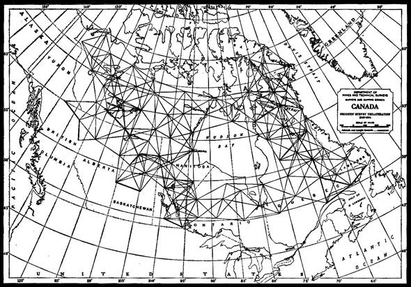
Map B2 : United States trilateration 1950 - Florida to Puerto Rico in 1950.
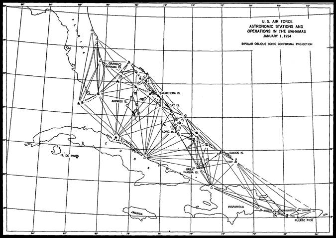
Map B3 : North African Tie 1952 - Crete and Rhodes to Libya and Egypt.
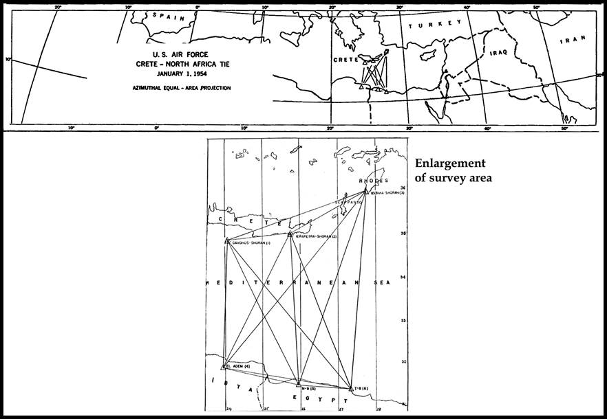
Map B4 : North Sea Tie 1952 - British Isles from Scotland to Norway.
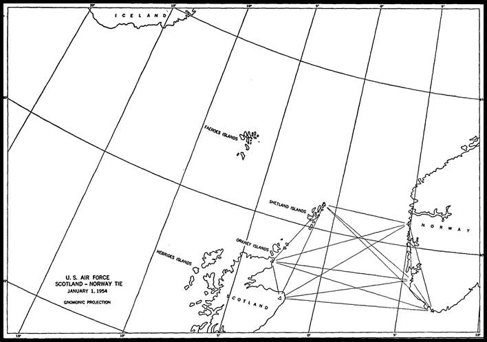
Map B5 : Southwest Pacific Survey (AF60-13) - Australia with Papua New Guinea, the Bismarck Archipelago, the Caroline and Marshall Islands, the Gilberts (Kiribati) and the Ellice (Tuvalu) Islands, and Fiji.
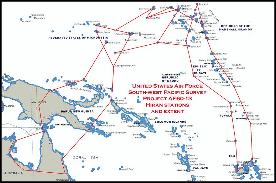
Graphic Survey of Radio and Radar Equipment
used by the Army Air Forces 1945
The first two pages describe the AN/APN-3, the airborne component of the Shoran system. The final two pages describe the AN/CPN-2, a Shoran ground responder unit. At least two responder units were required for line crossing operations.
|
|
|
|
|
|
|
|
|
This annexure was extracted from United States Army Air Forces: Graphic Survey of Radio and Radar Equipment used by the Army Air Forces 1945, Air Technical Service Command, AAF-MD-E89. |
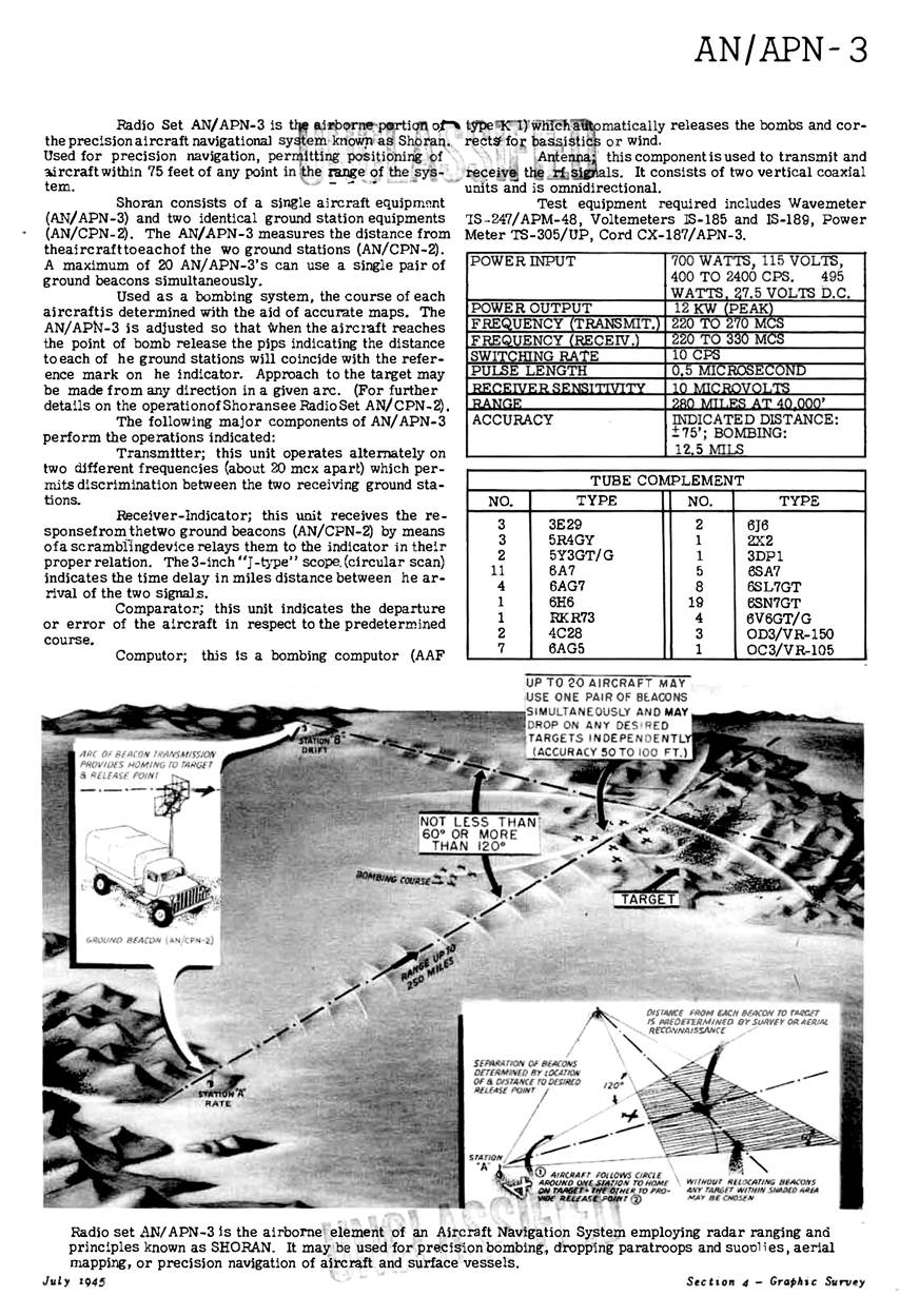
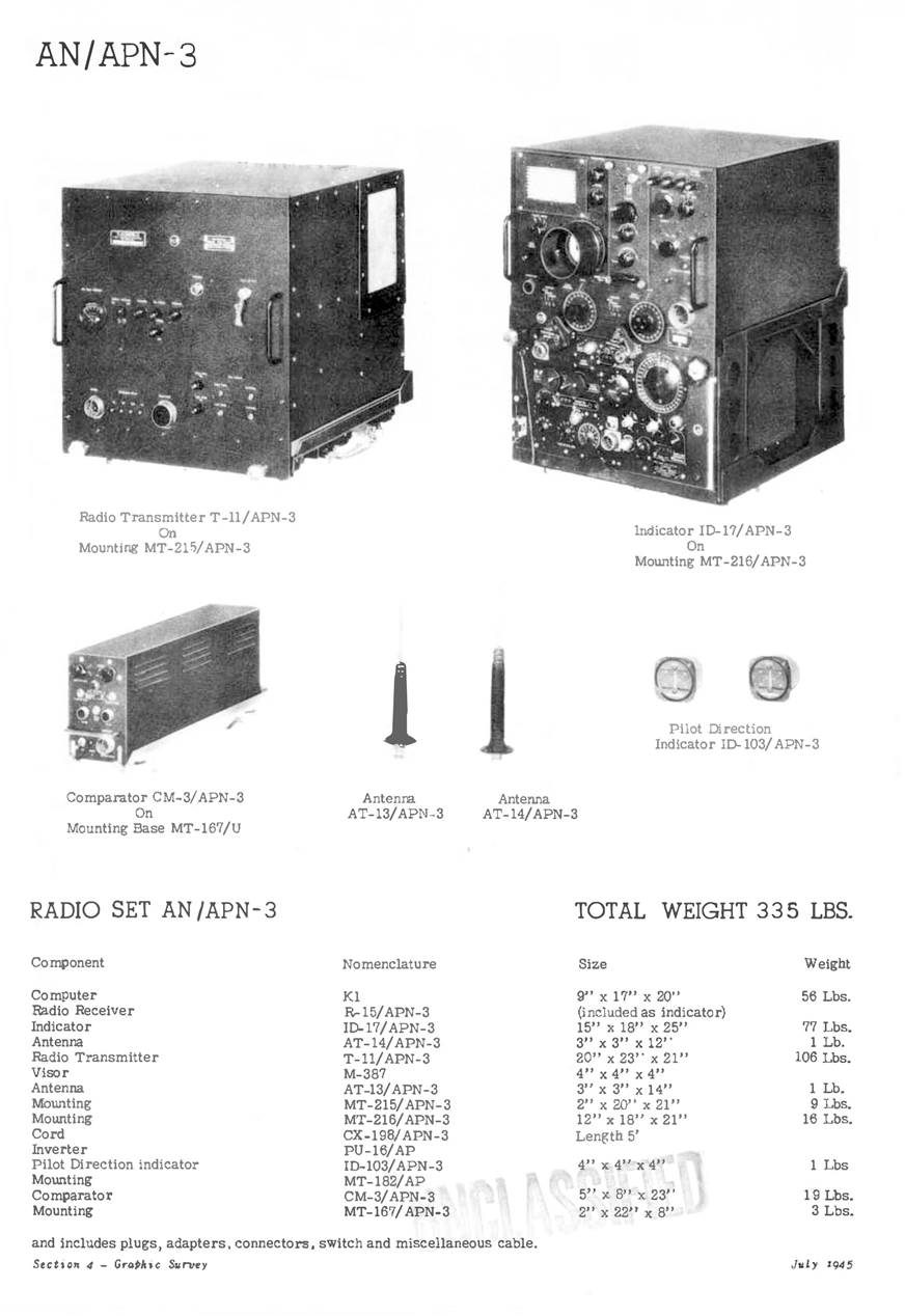
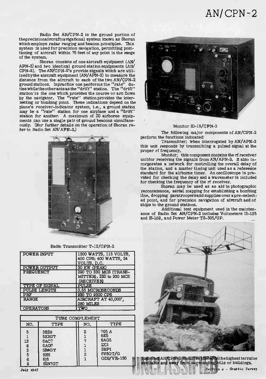
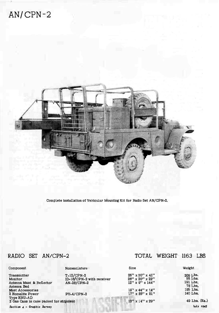
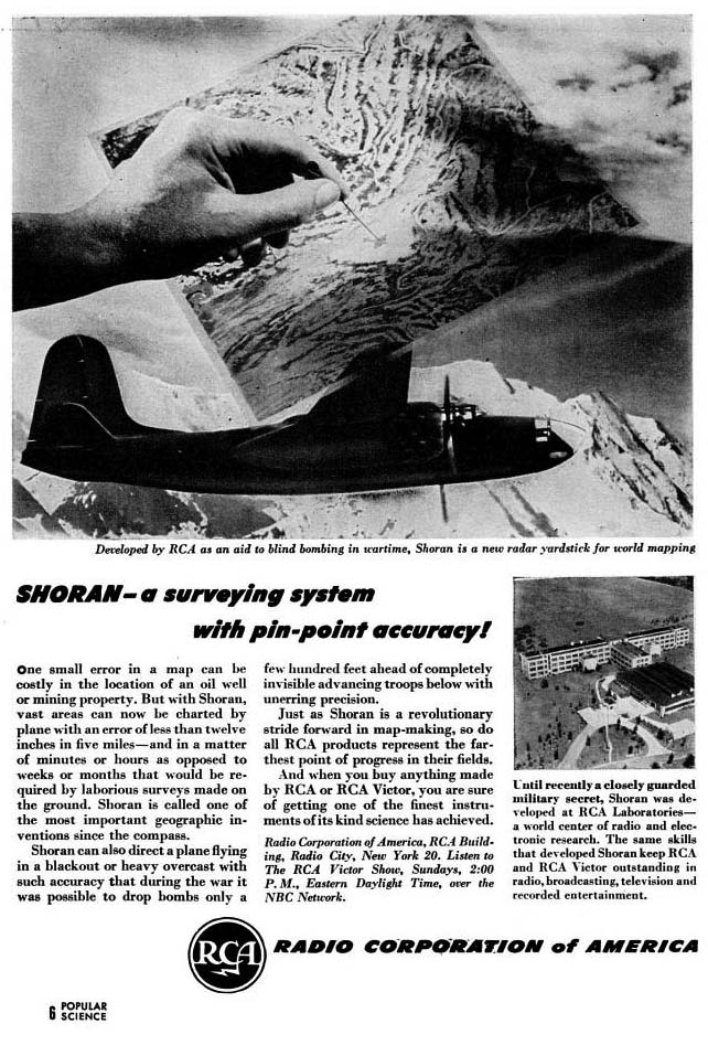
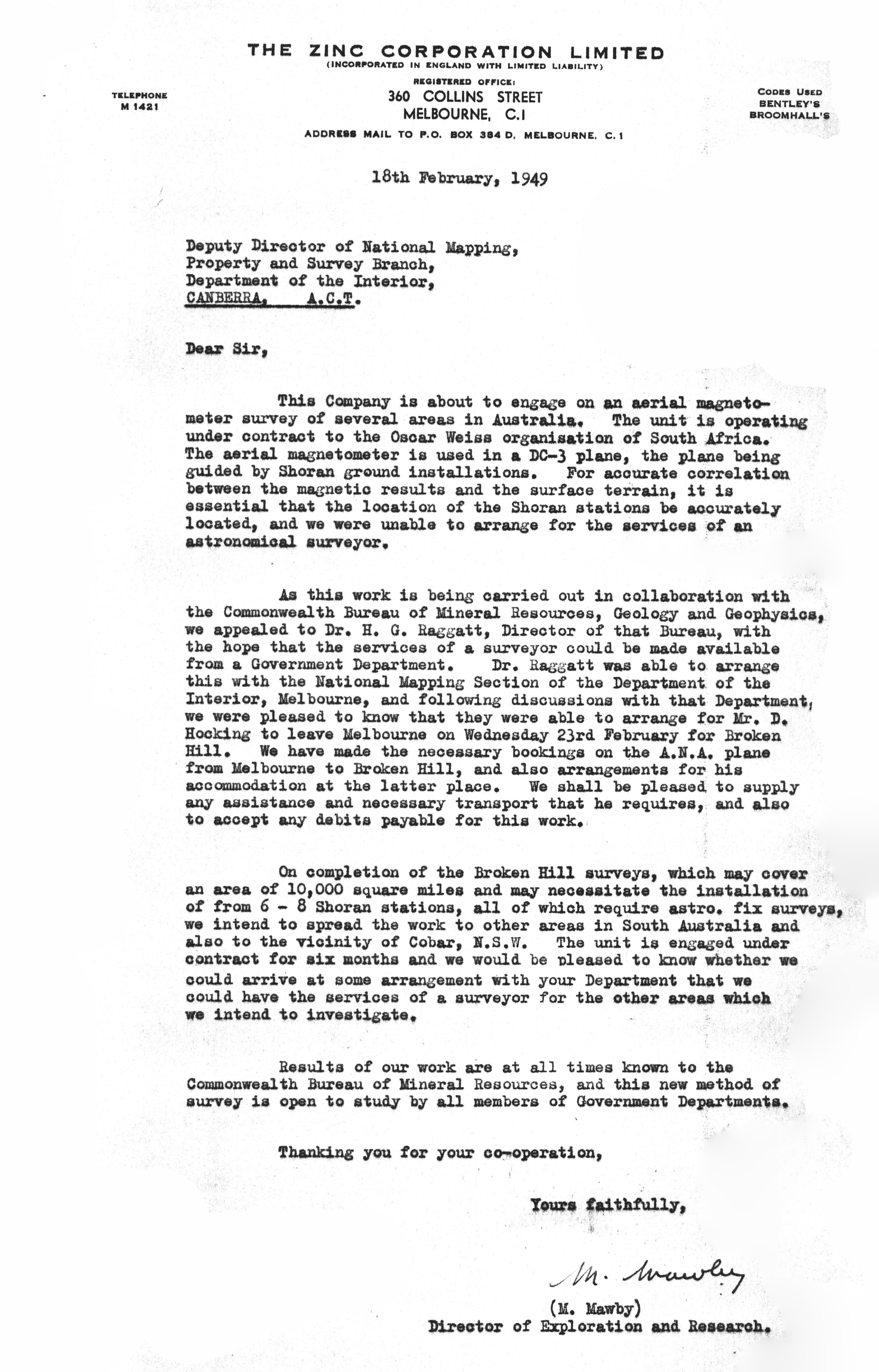
PROPOSAL FOR LINEAR EDGE CONTROL
OF PHOTOGRAMMETRIC BLOCKS
Generally, most systems used to obtain horizontal field control for photogrammetric mapping are directed to the acquisition of both X and Y coordinates, usually around the perimeter of a block. Whilst this is mandatory in completely uncontrolled areas, there are situations where the acquisition of either X or Y values could assist. Australia, for example is covered, or shortly will be, by a control grid on a one degree spacing, and there are indications that this spacing is too great to provide the whole perimeter control of block adjustment areas.
The grid, in itself, provides the essential control at the corners of mapping blocks, particularly if they are in suitable modules of 1:250,000 scale map areas. Having the corner control so readily available, it is only necessary to devise a scheme to restrain the bowing or bulging which would normally occur along the edges in between this basic one degree control. It is proposed to do this by figuratively stretching a string between these stations, i.e. by providing a series of control photographs along a straight line between the corner control points.
The spacing of the photographs along the piece of string is not critical, only the fact that they are on the straight line is important. In other words, it is proposed to control the perimeter bowing in photogrammetric block adjustments by using a series of points whose northings are accurately known, when spaced along a parallel, and whose eastings are known when spaced along a meridian. The requirement to provide one accurate ordinate only, instead of two, simplifies the field acquisition of control data very substantially.
To achieve this, it is proposed to position a laser beam drawn out into a vertical fan or wall, at an Aerodist station, and to direct it towards a second station, along an approximate azimuth derived from already established observations. The beam will miss the second station by an unknown amount, which could be up to 30 metres if the misalignment is about one minute of arc.
An aircraft carrying a vertical photogrammetric camera, camera attitude indicator (in development) and a laser sensor is then flown to approach the distant Aerodist station at right angles to the laser wall, as shown in the diagram below. To determine the azimuth correction of the laser curtain, the aircraft heading need only be approximate as the offset of the nadir point from the Aerodist station will be small and errors in heading not critical. On reaching the edge of the beam, the camera will be triggered by the laser light or pulse being detected by a sensor on the aircraft. The resultant photograph will record the relevant positions of the nadir point, the Aerodist station and the laser beam. A second picture can be exposed after a selected interval to provide stereo coverage.
These initial pictures will enable a photogrammetric evaluation of the misalignment of the laser beam to be made and to correct the subsequent series of photographs if necessary. Any number of subsequent control photographs can be provided by approaching the laser wall at right angles at selected intervals, the laser beam firing the camera as before. All of these points will lie on a straight line, and can be individually corrected to the line joining the two Aerodist stations.
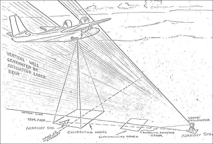
Looking at the proposal in more detail, the following observations can be made :
It does not appear that an excessively strong laser will be necessary. The Model 8 AGA Geodimeter, a small portable instrument, is capable of sensing a laser beam over a double path of 60 km or a total distance of 120 km. In this application a 5 milliwatt laser is diverged to 1.7 milliradians to enable the beam to be kept aligned with the retroprisms in spite of atmospheric effects. It is hoped that no divergence will be necessary in the proposed system, with the possibility of using an even smaller laser power source.
The sensing device in the same AGA Geodimeter is not very large and even if the airborne sensor has to be enlarged, it should still be possible to keep it relatively small. The size of this sensor is discussed in detail further on.
Aerodist stations are cleared to have an unobstructed view above 1.5 degrees elevation. As the proposed flying height of the camera aircraft is a maximum of 3,000 metres and the maximum range is about 100 km, this should not present any difficulty.
The laser beam can be drawn out into a fan by two means either optically; by using a cylindrical astigmatising lens or mechanically; by a number of tangential mirrors on the periphery of a rotating wheel. To ensure that a laser pulse reaches the aircraft camera sensor to trigger the camera at the right instant, the size of the sensor must be based on the number of mirrors, their rotational speed, and the speed of the aircraft. Thirty-six mirrors mounted on a wheel rotating at 16,000 rpm would mean the transmission of 9,600 pulses every second. However, the aircraft sensor would also be moving at about 50 metres/second and would advance some 5 millimetres between pulses. Thus to register a pulse, the aircraft sensor would have to be larger than 5 millimetres to ensure that sufficient pulses would trigger the camera.
The verticality of the laser wall should not present a problem as a dislevelment of even 20 seconds of arc, representing 0.3 metres at the proposed flying height, could be tolerated. Gravity effects would be smaller still.
The system may be affected to some extent by prevailing conditions of visibility. However, because the photographs produced are to be used for control purposes only, they do not need to be of mapping quality. Advantage can therefore be taken of the more stable visibility conditions prevailing early and late in the day even though shadow lengths may be longer than desirable. Some detailed scheduling of flying times will be necessary to maintain uninterrupted production, and to take advantage of the most favourable flying conditions.
It is envisaged that large areas of Australia where the road systems are adequate, could be covered by transporting the laser by vehicle, with the camera and sensor in a light twin engined aircraft. In less developed areas, the laser generator would probably be best transported in a small helicopter. Each set up would provide 400 km of linear control photographs in the four cardinal directions, with the result that only alternative setups would be required through the basic control grid. In addition to providing the peripheral control, supplementary lines would reach into the area at right angles to the surround, adding even further horizontal control to the photogrammetric block.
A photogrammetric block of 12 x 1:250,000 scale map sheet areas could be controlled by occupying just 9 stations, as shown in the diagram below, and provide 3,600 kilometres of control in a short space of time.
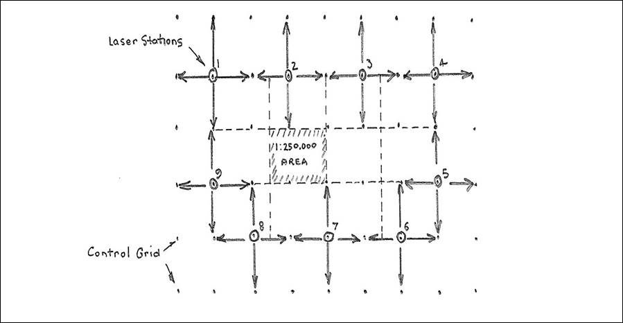
This annexure is a copy of an internal working paper developed by the Control Survey Branch, Division of National Mapping, Melbourne circa 1975.